# Technical Data Extraction: Performance vs. Effective Context Length
This document provides a detailed extraction of the data and trends presented in the two-panel line chart comparing different retrieval and generation configurations.
## 1. General Layout and Metadata
* **Image Type:** Two-panel line graph with logarithmic x-axis.
* **Y-Axis (Both Panels):** "Normalized Performance" (Linear scale from -3 to +3, with major gridlines at intervals of 1.0).
* **X-Axis (Both Panels):** "Effective Context Length" (Logarithmic scale from $10^2$ to $10^6+$).
* **Visual Elements:**
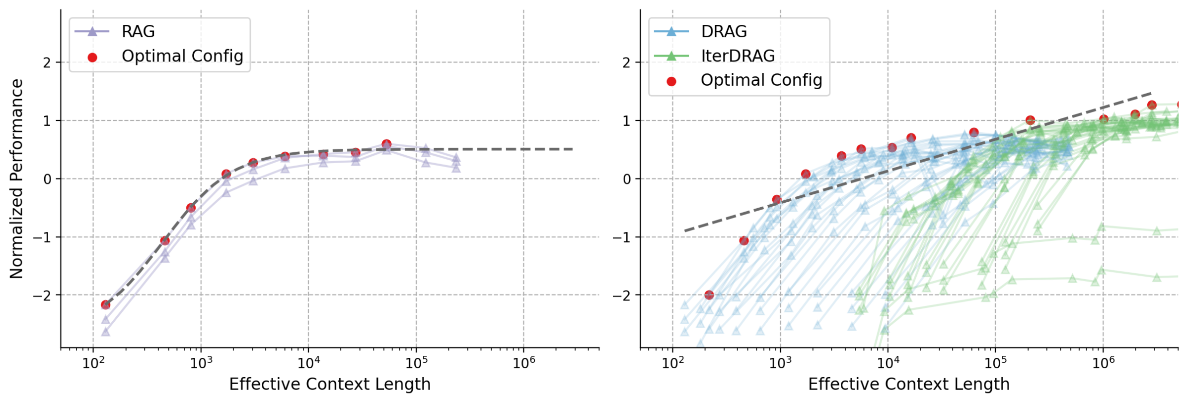
* **Dashed Grey Line:** Represents the theoretical or empirical "frontier" of optimal performance across context lengths.
* **Red Dots:** Labeled as "Optimal Config," these mark the peak performance points for specific context length intervals.
* **Faded Lines with Triangles:** Represent individual experimental runs/configurations.
---
## 2. Left Panel: RAG Performance
### Component Isolation: Left Chart
* **Legend Location:** Top-left $[x \approx 0.05, y \approx 0.9]$.
* **Series 1 (Purple Triangles):** **RAG**. Multiple faded purple lines showing various RAG configurations.
* **Series 2 (Red Circles):** **Optimal Config**. Points following the upper boundary of the RAG configurations.
### Trend Analysis: RAG
The RAG performance shows a steep logarithmic growth starting from approximately -2.5 at $10^2$ context length. The performance plateaus significantly after $10^4$ context length, reaching a maximum normalized performance of approximately 0.5.
### Data Points (Optimal Config - RAG)
| Effective Context Length (Approx.) | Normalized Performance (Approx.) | Trend Observation |
| :--- | :--- | :--- |
| $1.2 \times 10^2$ | -2.2 | Rapid ascent |
| $5 \times 10^2$ | -1.1 | Rapid ascent |
| $10^3$ | -0.5 | Decelerating growth |
| $2 \times 10^3$ | 0.1 | Approaching plateau |
| $6 \times 10^3$ | 0.4 | Plateau entry |
| $10^4$ to $10^5$ | 0.4 to 0.6 | Stable plateau |
---
## 3. Right Panel: DRAG and IterDRAG Performance
### Component Isolation: Right Chart
* **Legend Location:** Top-left $[x \approx 0.55, y \approx 0.9]$.
* **Series 1 (Blue Triangles):** **DRAG**. Faded blue lines representing various DRAG configurations.
* **Series 2 (Green Triangles):** **IterDRAG**. Faded green lines representing iterative DRAG configurations.
* **Series 3 (Red Circles):** **Optimal Config**. Points marking the highest performance achieved at various context lengths across both methods.
### Trend Analysis: DRAG vs. IterDRAG
* **DRAG (Blue):** Dominates the lower context lengths ($10^2$ to $10^4$). It shows a similar growth curve to RAG but maintains a higher trajectory, crossing the 0.0 performance mark around $3 \times 10^3$.
* **IterDRAG (Green):** Becomes relevant at higher context lengths ($>10^4$). While individual runs vary wildly, the "Optimal Config" points in the $10^5$ to $10^6$ range are driven by these configurations.
* **Overall Frontier (Dashed Line):** Unlike the RAG panel which plateaus, the DRAG/IterDRAG frontier continues to climb steadily, exceeding a normalized performance of 1.0 as context length approaches $10^6$.
### Data Points (Optimal Config - DRAG/IterDRAG)
| Effective Context Length (Approx.) | Normalized Performance (Approx.) | Series Source |
| :--- | :--- | :--- |
| $2 \times 10^2$ | -2.0 | DRAG |
| $4 \times 10^2$ | -1.1 | DRAG |
| $10^3$ | -0.4 | DRAG |
| $2 \times 10^3$ | 0.1 | DRAG |
| $5 \times 10^3$ | 0.5 | DRAG |
| $10^4$ | 0.6 | DRAG |
| $6 \times 10^4$ | 0.8 | DRAG/IterDRAG |
| $2 \times 10^5$ | 1.0 | IterDRAG |
| $10^6$ | 1.1 | IterDRAG |
| $3 \times 10^6$ | 1.3 | IterDRAG |
---
## 4. Comparative Summary
* **Scaling Ceiling:** RAG (Left) hits a performance ceiling of $\approx 0.5$ at $10^4$ context length. In contrast, DRAG/IterDRAG (Right) breaks this ceiling, reaching $>1.0$ performance as context length scales toward $10^6$.
* **Configuration Density:** The right panel shows a much higher density of experimental configurations (faded lines), particularly for IterDRAG at high context lengths, indicating a larger search space or higher sensitivity to parameters at scale.
* **Optimal Frontier:** The dashed grey line in the right panel has a positive slope throughout the entire x-axis range, whereas the left panel's frontier becomes horizontal (slope $\approx 0$) after $10^4$.