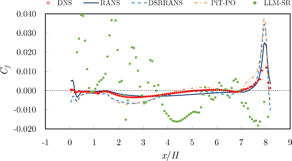
\n ## Line Plot: Comparison of C_f Predictions Across Different CFD Methods ### Overview The image is a scientific line plot comparing the skin friction coefficient (C_f) predictions from five different computational fluid dynamics (CFD) methods or models as a function of the normalized streamwise position (x/H). The plot serves as a benchmark, likely against a high-fidelity reference solution (DNS), to evaluate the accuracy of various turbulence modeling or simulation approaches. ### Components/Axes * **Chart Type:** 2D line plot with overlaid scatter points. * **X-Axis:** * **Label:** `x/H` (Normalized streamwise coordinate, likely distance from a reference point divided by a characteristic height H). * **Scale:** Linear, ranging from -1 to 9. * **Major Ticks:** At integer intervals: -1, 0, 1, 2, 3, 4, 5, 6, 7, 8, 9. * **Y-Axis:** * **Label:** `C_f` (Skin friction coefficient). * **Scale:** Linear, ranging from -0.020 to 0.040. * **Major Ticks:** At intervals of 0.010: -0.020, -0.010, 0.000, 0.010, 0.020, 0.030, 0.040. * **Reference Line:** A horizontal dashed black line at `C_f = 0.000`. * **Legend:** Positioned at the top center of the plot area. It contains five entries: 1. `DNS` (Direct Numerical Simulation): Represented by red diamond markers (◇). 2. `RANS` (Reynolds-Averaged Navier-Stokes): Represented by a solid dark blue line. 3. `DSRRANS` (Likely a specific RANS variant): Represented by a dashed light blue line. 4. `PiT-PO` (Likely a specific model or method): Represented by a dash-dot orange line. 5. `LLM-SR` (Likely a machine learning-based super-resolution or correction method): Represented by solid green circle markers (●). ### Detailed Analysis **Trend Verification & Data Point Extraction (Approximate Values):** 1. **DNS (Red Diamonds):** * **Trend:** The reference data remains very close to `C_f = 0` for most of the domain (`x/H` from 0 to ~7.5). It shows a sharp, narrow positive peak centered near `x/H = 8.0`, reaching a maximum `C_f` of approximately **0.012**. The data points are densely clustered along the zero line and around the peak. * **Key Points:** `(0, ~0.000)`, `(1, ~0.000)`, `(4, ~0.000)`, `(7.5, ~0.000)`, `(8.0, ~0.012)`, `(8.2, ~0.000)`. 2. **RANS (Solid Dark Blue Line):** * **Trend:** Starts with a small positive value near `x/H=0`, dips slightly negative between `x/H=0.5` and `x/H=1.5`, then follows a smooth, slightly negative curve until `x/H=7`. It then rises sharply to form a peak that is **broader and lower** than the DNS peak, reaching a maximum of approximately **0.025** at `x/H ≈ 8.0`. It then drops sharply. * **Key Points (Line):** `(0, ~0.005)`, `(1, ~-0.002)`, `(4, ~-0.003)`, `(7, ~-0.001)`, `(8.0, ~0.025)`, `(8.5, ~0.000)`. 3. **DSRRANS (Dashed Light Blue Line):** * **Trend:** Shows more oscillation than RANS. It starts negative near `x/H=0`, has a small positive bump around `x/H=1`, then dips to a minimum near `x/H=2.5`. It recovers to near zero by `x/H=5` and follows a path similar to RANS towards the peak. Its peak at `x/H ≈ 8.0` is **slightly higher and sharper** than RANS, reaching approximately **0.035**. * **Key Points (Line):** `(0, ~-0.005)`, `(1, ~0.001)`, `(2.5, ~-0.007)`, `(5, ~0.000)`, `(8.0, ~0.035)`, `(8.5, ~-0.015)`. 4. **PiT-PO (Dash-Dot Orange Line):** * **Trend:** Follows a path very similar to DSRRANS in the region `x/H < 7`. However, its peak at `x/H ≈ 8.0` is the **highest and sharpest** among all models, reaching a maximum `C_f` of approximately **0.038**. It then drops precipitously. * **Key Points (Line):** `(0, ~-0.005)`, `(2.5, ~-0.007)`, `(7, ~0.002)`, `(8.0, ~0.038)`, `(8.2, ~0.000)`. 5. **LLM-SR (Green Dots):** * **Trend:** This data series is highly scattered and does not follow a smooth curve. It shows significant deviations from the other models and the DNS reference. * **Region `x/H = 0 to 4`:** Points are widely scattered between `C_f ≈ -0.015` and `C_f ≈ 0.040`, with no clear trend. Many points lie far above the DNS/RANS lines. * **Region `x/H = 4 to 6`:** Points form a distinct, smooth **negative trough**, reaching a minimum of approximately **-0.016** near `x/H = 4.5`. This is a major deviation from all other models, which are near zero here. * **Region `x/H = 6 to 9`:** Points become scattered again, mostly negative, with a cluster near the DNS peak at `x/H=8` but also many points far below it (down to `C_f ≈ -0.018`). * **Key Observations:** The LLM-SR data suggests either a very different physical prediction, significant noise, or that it represents a different type of output (e.g., point-wise corrections or errors) rather than a continuous model prediction. ### Key Observations 1. **Peak Discrepancy at x/H ≈ 8:** All RANS-based models (RANS, DSRRANS, PiT-PO) predict a positive `C_f` peak at `x/H ≈ 8`, consistent with the DNS location. However, they all **overpredict the magnitude** of the peak compared to DNS. The order of overprediction is: PiT-PO > DSRRANS > RANS. 2. **Upstream Behavior:** In the region `x/H < 7`, the DNS data is essentially zero. The RANS models show small negative values, with DSRRANS and PiT-PO showing a more pronounced negative dip around `x/H=2.5`. 3. **Anomalous LLM-SR Data:** The LLM-SR data is the most striking outlier. Its smooth, deep negative trough between `x/H=4` and `x/H=6` is not present in any other dataset. Its high scatter elsewhere suggests it may not be a direct competitor model in the same category as the others, or it represents a fundamentally different approach with high variance. 4. **Model Similarity:** The DSRRANS and PiT-PO lines are nearly identical for `x/H < 7`, diverging only in the magnitude of the final peak. ### Interpretation This plot is a classic model validation exercise in computational fluid dynamics. The DNS data serves as the "ground truth." The comparison reveals: * **Standard RANS Limitations:** The basic RANS model captures the qualitative feature (a peak at `x/H=8`) but smears it out (broader, lower peak) and introduces a slight negative `C_f` upstream, which is not present in the DNS. This is typical of RANS models' difficulty with separated flows or complex boundary layer interactions. * **Improved RANS Variants:** DSRRANS and PiT-PO appear to be attempts to improve upon standard RANS. They sharpen the peak (bringing it closer to the DNS shape) but at the cost of significantly overpredicting its magnitude. Their identical upstream behavior suggests they share a common base formulation. * **Machine Learning Approach (LLM-SR):** The LLM-SR data is puzzling. If it represents a direct prediction of `C_f`, it performs poorly, showing large errors and spurious features (the deep trough). However, it's possible this plot shows something else, like the *correction* applied by the LLM or its *predicted error field*. The high scatter could indicate a point-wise, non-physics-constrained method. Its value lies not in matching the curve, but perhaps in identifying regions of high model uncertainty (e.g., the scattered points upstream and the distinct pattern in the mid-section). * **Flow Physics Implication:** The sharp peak in `C_f` at `x/H=8` likely corresponds to a **flow reattachment point** or the end of a separation bubble. The negative `C_f` values predicted by some models upstream would indicate reverse flow (separation), which the DNS shows does not occur (C_f ≥ 0). The models' struggle to accurately predict both the absence of separation upstream and the precise reattachment peak highlights a key challenge in turbulence modeling for this flow configuration.