## [Bar Chart with Table Overlay]: Probability Distribution of 5-Bit Binary States (Boltzmann vs. Measured)
### Overview
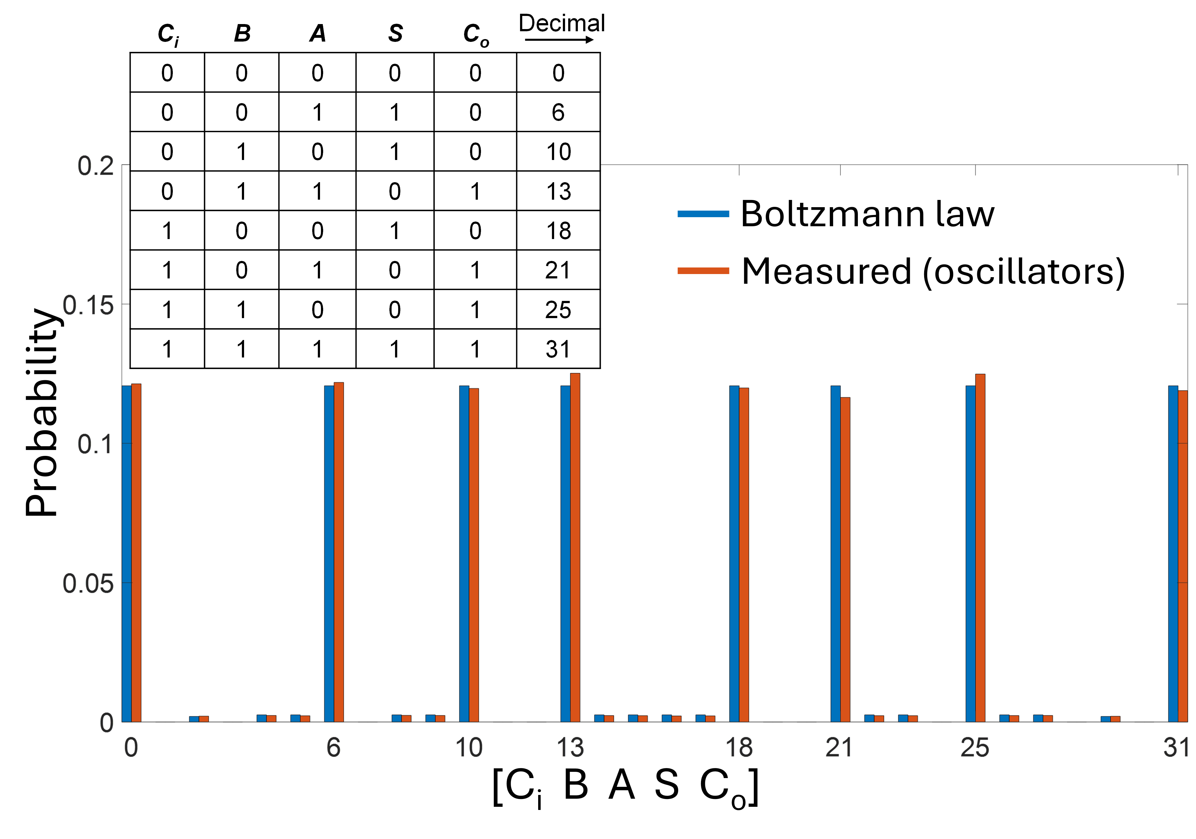
The image presents a bar graph comparing the probability of 5-bit binary states (represented as \([C_i\ B\ A\ S\ C_o]\)) between the **Boltzmann law** (theoretical, blue bars) and **measured data from oscillators** (experimental, orange bars). A table in the top-left corner maps 5-bit binary values to their decimal equivalents, defining the states plotted on the x-axis.
### Components/Axes
- **Y-axis**: Labeled "Probability" with ticks at \(0, 0.05, 0.1, 0.15, 0.2\).
- **X-axis**: Labeled \([C_i\ B\ A\ S\ C_o]\) with tick marks at decimal values \(0, 6, 10, 13, 18, 21, 25, 31\) (matching the table’s "Decimal" column).
- **Legend**: Top-right, with:
- Blue: "Boltzmann law" (theoretical probability).
- Orange: "Measured (oscillators)" (experimental probability).
- **Table (Top-Left)**: Columns: \(C_i, B, A, S, C_o, \text{Decimal}\). Rows (binary → decimal):
| \(C_i\) | \(B\) | \(A\) | \(S\) | \(C_o\) | Decimal |
|---------|-------|-------|-------|---------|---------|
| 0 | 0 | 0 | 0 | 0 | 0 |
| 0 | 0 | 1 | 1 | 0 | 6 |
| 0 | 1 | 0 | 1 | 0 | 10 |
| 0 | 1 | 1 | 0 | 1 | 13 |
| 1 | 0 | 0 | 1 | 0 | 18 |
| 1 | 0 | 1 | 0 | 1 | 21 |
| 1 | 1 | 0 | 0 | 1 | 25 |
| 1 | 1 | 1 | 1 | 1 | 31 |
### Detailed Analysis
- **Bar Heights (Probability)**:
For each decimal state (x-axis tick: \(0, 6, 10, 13, 18, 21, 25, 31\)):
- Blue (Boltzmann) and orange (Measured) bars have nearly identical heights, approximately \(0.12–0.13\) (visually between \(0.1\) and \(0.15\), closer to \(0.125\)).
- Between these main ticks (e.g., between \(0\) and \(6\), \(6\) and \(10\), etc.), small blue/orange bars (near \(0\) probability) indicate negligible probability for intermediate states.
### Key Observations
1. **Theory-Experiment Alignment**: The Boltzmann law (blue) and measured (orange) bars are nearly identical in height for all plotted states, suggesting the oscillator system’s probability distribution closely matches the Boltzmann distribution.
2. **Negligible Intermediate States**: Small bars between main ticks (e.g., between \(0\) and \(6\)) have near-zero probability, meaning these binary states are rarely observed.
3. **State Selection**: The system preferentially occupies the 5-bit states listed in the table (with non-negligible probability), while other states are rarely occupied.
### Interpretation
- **Boltzmann Law Validation**: The close match between theoretical (Boltzmann) and measured probabilities confirms the oscillator system’s behavior follows the Boltzmann law (a key result in statistical mechanics, relating energy states to probability).
- **State Stability**: The plotted states (e.g., \(0, 6, 10, 13, 18, 21, 25, 31\)) likely correspond to lower-energy configurations (consistent with Boltzmann’s energy-probability relationship), explaining their higher probability.
- **Practical Implication**: The system’s measured probabilities align with theoretical expectations, validating the use of Boltzmann statistics to model its behavior. The negligible probability of intermediate states suggests a discrete, well-defined set of stable configurations.
This analysis confirms the oscillator system’s probability distribution is consistent with the Boltzmann law, with preferential occupation of specific 5-bit binary states.