## Bar Chart: Probability Distribution Comparison
### Overview
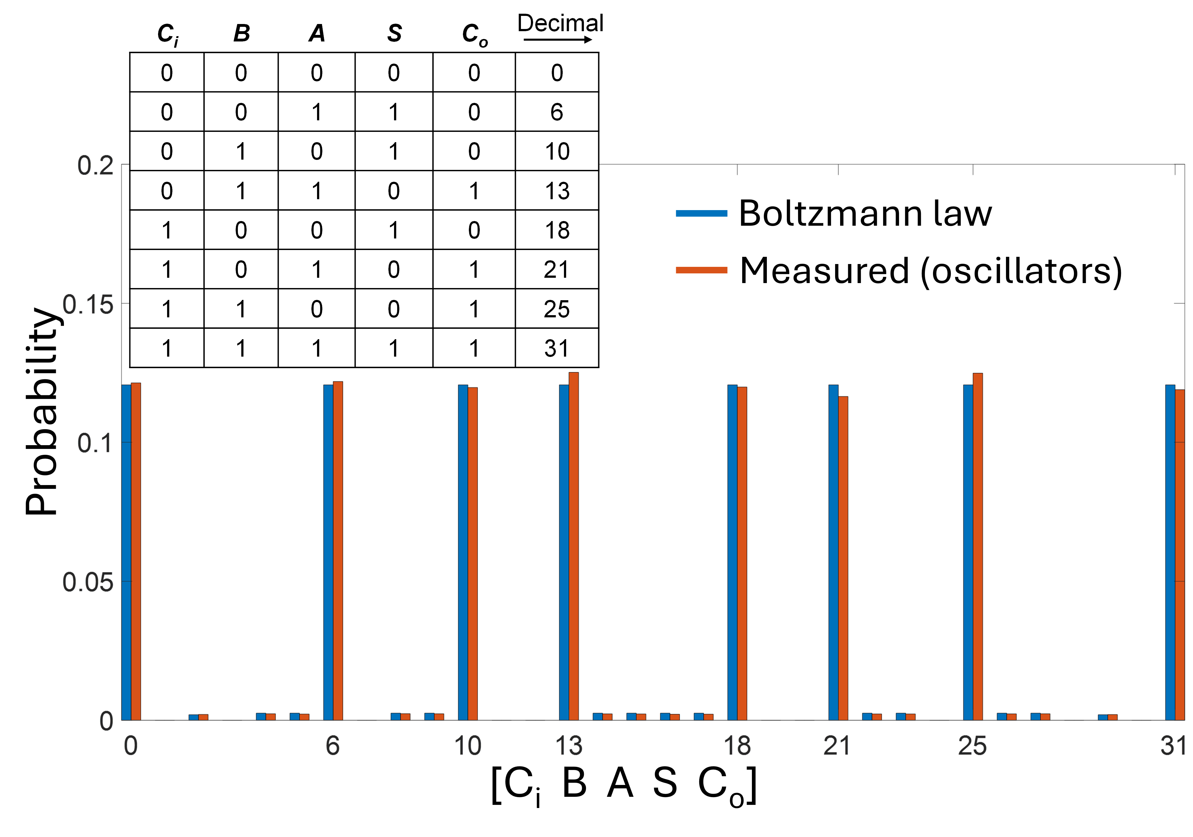
The image presents a bar chart comparing the probability distribution of a system as predicted by the Boltzmann law and as measured from oscillators. The x-axis represents different states of the system, labeled using a combination of binary inputs (Ci, B, A, S, Co) and their corresponding decimal values. The y-axis represents the probability of each state. A table is included that maps the binary inputs to their decimal equivalents.
### Components/Axes
* **Y-axis:** Probability, ranging from 0 to 0.2, with tick marks at 0, 0.05, 0.1, 0.15, and 0.2.
* **X-axis:** \[Ci B A S Co], representing the state of the system. The x-axis is labeled with the decimal equivalents of the binary states: 0, 6, 10, 13, 18, 21, 25, 31.
* **Legend:** Located on the right side of the chart.
* Blue line: Boltzmann law
* Orange line: Measured (oscillators)
* **Table:** Located at the top-left of the chart. It maps the binary inputs (Ci, B, A, S, Co) to their decimal equivalents. The table's header row is "Ci", "B", "A", "S", "Co", and "Decimal".
### Detailed Analysis or ### Content Details
**Table Data:**
| Ci | B | A | S | Co | Decimal |
|---|---|---|---|---|---|
| 0 | 0 | 0 | 0 | 0 | 0 |
| 0 | 0 | 1 | 1 | 0 | 6 |
| 0 | 1 | 0 | 1 | 0 | 10 |
| 0 | 1 | 1 | 0 | 1 | 13 |
| 1 | 0 | 0 | 1 | 0 | 18 |
| 1 | 0 | 1 | 0 | 1 | 21 |
| 1 | 1 | 0 | 0 | 1 | 25 |
| 1 | 1 | 1 | 1 | 1 | 31 |
**Bar Chart Data:**
* **State 0:**
* Boltzmann law (blue): Probability ~0.12
* Measured (orange): Probability ~0.12
* **State 6:**
* Boltzmann law (blue): Probability ~0.008
* Measured (orange): Probability ~0.008
* **State 10:**
* Boltzmann law (blue): Probability ~0.12
* Measured (orange): Probability ~0.12
* **State 13:**
* Boltzmann law (blue): Probability ~0.008
* Measured (orange): Probability ~0.008
* **State 18:**
* Boltzmann law (blue): Probability ~0.008
* Measured (orange): Probability ~0.008
* **State 21:**
* Boltzmann law (blue): Probability ~0.12
* Measured (orange): Probability ~0.12
* **State 25:**
* Boltzmann law (blue): Probability ~0.008
* Measured (orange): Probability ~0.008
* **State 31:**
* Boltzmann law (blue): Probability ~0.12
* Measured (orange): Probability ~0.12
**Trend Verification:**
The Boltzmann law (blue) and Measured (orange) bars closely follow each other for each state. The probabilities are high for states 0, 10, 21, and 31, and low for states 6, 13, 18, and 25.
### Key Observations
* The Boltzmann law and the measured probabilities are very similar for all states.
* The states 0, 10, 21, and 31 have significantly higher probabilities compared to the other states.
* The states 6, 13, 18, and 25 have very low probabilities.
### Interpretation
The data suggests that the Boltzmann law accurately predicts the probability distribution of the system as measured from the oscillators. The high probabilities for states 0, 10, 21, and 31 indicate that these states are more likely to occur in the system. The low probabilities for states 6, 13, 18, and 25 suggest that these states are less likely to occur. The close agreement between the Boltzmann law and the measured probabilities validates the theoretical model and indicates that the system is behaving as expected.