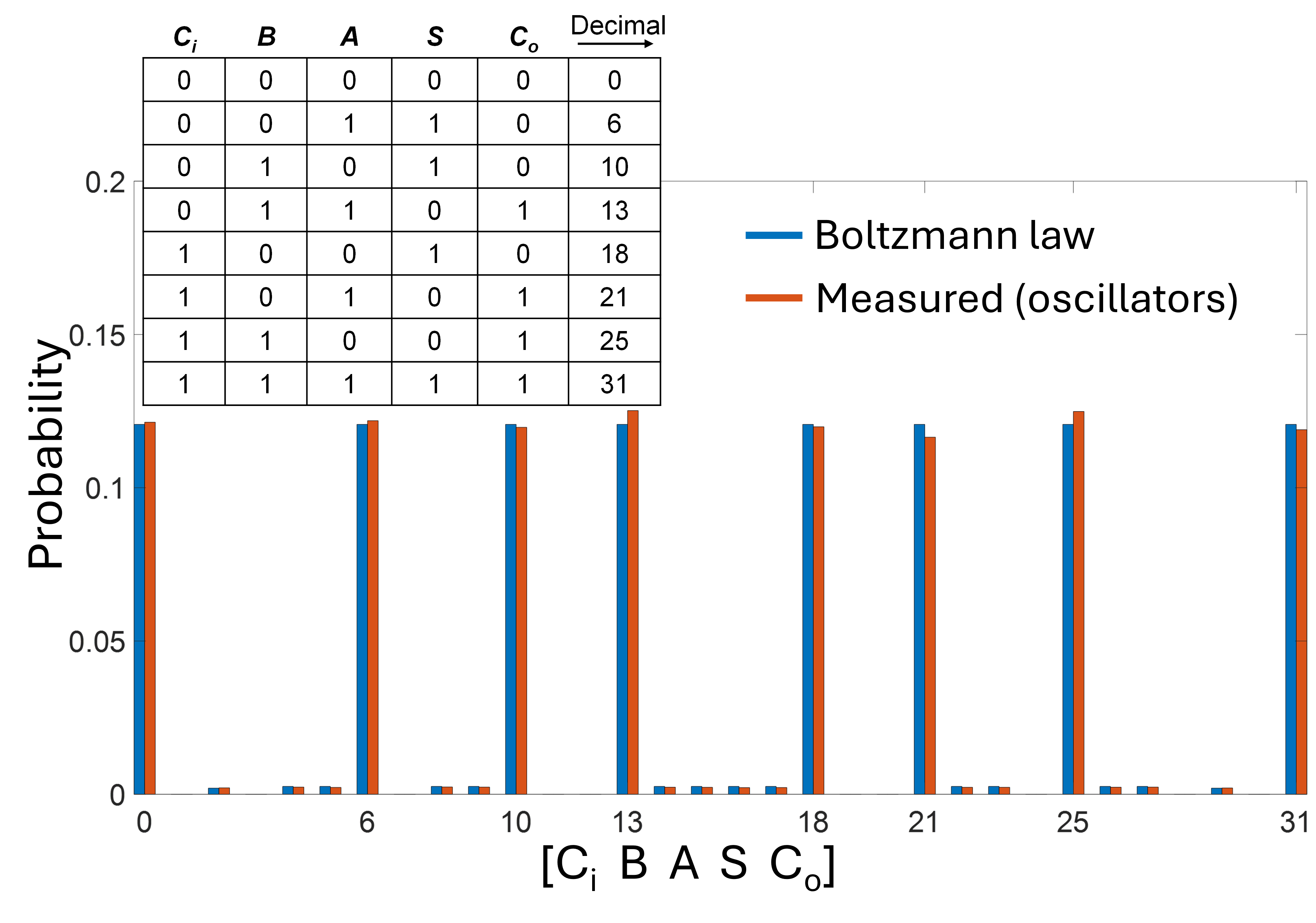
\n ## Bar Chart: Probability Distribution Comparison - Boltzmann Law vs. Measured Oscillators ### Overview This image presents a bar chart comparing the probability distribution predicted by the Boltzmann law with the probability distribution measured from oscillators. The chart displays probability on the y-axis against a discrete variable represented by [Cᵢ B A S C₀] on the x-axis. A table is included at the top-left of the chart, mapping binary values (Cᵢ, B, A, S, C₀) to decimal values. ### Components/Axes * **X-axis:** Labeled "[Cᵢ B A S C₀]", representing a discrete variable. The axis is marked with values 0, 6, 10, 13, 18, 21, 25, and 31. * **Y-axis:** Labeled "Probability", with a scale ranging from 0 to 0.22. * **Legend:** Located in the top-right corner. * "Boltzmann law" - represented by a blue line/bars. * "Measured (oscillators)" - represented by an orange/red line/bars. * **Table:** Located in the top-left corner. Columns labeled Cᵢ, B, A, S, C₀, and Decimal. ### Detailed Analysis The chart consists of paired bars for each x-axis value, representing the Boltzmann law prediction and the measured oscillator data. * **X = 0:** Boltzmann law probability is approximately 0.002. Measured probability is approximately 0.003. * **X = 6:** Boltzmann law probability is approximately 0.12. Measured probability is approximately 0.125. * **X = 10:** Boltzmann law probability is approximately 0.12. Measured probability is approximately 0.115. * **X = 13:** Boltzmann law probability is approximately 0.02. Measured probability is approximately 0.015. * **X = 18:** Boltzmann law probability is approximately 0.12. Measured probability is approximately 0.115. * **X = 21:** Boltzmann law probability is approximately 0.02. Measured probability is approximately 0.01. * **X = 25:** Boltzmann law probability is approximately 0.02. Measured probability is approximately 0.015. * **X = 31:** Boltzmann law probability is approximately 0.005. Measured probability is approximately 0.01. The table provides the following mapping: | Cᵢ | B | A | S | C₀ | Decimal | |---|---|---|---|---|---| | 0 | 0 | 0 | 0 | 0 | 0 | | 0 | 0 | 1 | 1 | 0 | 6 | | 0 | 1 | 0 | 1 | 0 | 10 | | 0 | 1 | 1 | 0 | 1 | 13 | | 1 | 0 | 0 | 0 | 0 | 18 | | 1 | 0 | 1 | 0 | 1 | 21 | | 1 | 1 | 0 | 0 | 1 | 25 | | 1 | 1 | 1 | 1 | 1 | 31 | ### Key Observations * The Boltzmann law and measured probabilities are generally in good agreement, particularly at x = 6 and x = 10. * There are slight discrepancies at x = 13, x = 21, and x = 25, where the measured probabilities are lower than the Boltzmann law predictions. * The probability values are highest at x = 6 and x = 10, and decrease significantly for other values. * The probability values are very low at x = 0, x = 13, x = 21, x = 25, and x = 31. ### Interpretation The chart demonstrates a comparison between the theoretical probability distribution predicted by the Boltzmann law and the experimentally measured probability distribution of oscillators. The close agreement between the two distributions suggests that the Boltzmann law is a reasonable model for the behavior of these oscillators. The slight discrepancies observed at certain values may indicate deviations from the assumptions underlying the Boltzmann law, or may be due to experimental error. The binary representation and its decimal equivalent suggest that the variable [Cᵢ B A S C₀] represents a state or configuration of the oscillators, and the probability distribution describes the likelihood of observing each state. The peaks at x=6 and x=10 indicate that these states are the most probable configurations for the oscillators. The low probabilities at the extreme values (0, 31) suggest that these configurations are rare.