## Line Charts: Model Performance vs. Compute and Data Efficiency
### Overview
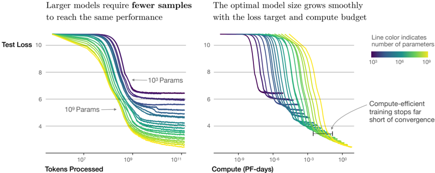
The image contains two side-by-side line charts comparing model performance (test loss) across different parameter sizes (10³ to 10⁹ parameters) under varying computational and data constraints. The left chart focuses on data efficiency (tokens processed), while the right chart emphasizes computational efficiency (PF-days). Both charts demonstrate how larger models achieve better performance with fewer resources.
### Components/Axes
**Left Chart: Test Loss vs. Tokens Processed**
- **X-axis**: Tokens Processed (log scale: 10⁷ to 10¹¹)
- **Y-axis**: Test Loss (linear scale: 4 to 10)
- **Legend**: Line color gradient indicates parameter count (purple = 10³, yellow = 10⁹)
- **Annotations**:
- Arrow pointing to "10³ Params" near the top-left
- Arrow pointing to "10⁹ Params" near the bottom-left
**Right Chart: Test Loss vs. Compute (PF-days)**
- **X-axis**: Compute (PF-days, log scale: 10⁻⁹ to 10⁰)
- **Y-axis**: Test Loss (linear scale: 4 to 10)
- **Legend**: Same color gradient as left chart (parameters)
- **Annotations**:
- Arrow pointing to "Compute-efficient training stops far short of convergence" near the bottom-right
### Detailed Analysis
**Left Chart Trends**:
- All lines slope downward, indicating improved performance (lower test loss) as tokens processed increase.
- Larger models (yellow/green lines) achieve lower test loss at earlier token counts compared to smaller models (purple/blue lines).
- Example: At ~10⁹ tokens, 10⁹-parameter models (yellow) reach ~6 test loss, while 10³-parameter models (purple) require ~10¹¹ tokens to reach ~8 test loss.
**Right Chart Trends**:
- All lines slope downward, showing improved performance with increased compute.
- Larger models (yellow/green) achieve lower test loss at lower compute budgets compared to smaller models.
- Example: At ~10⁻³ PF-days, 10⁹-parameter models reach ~5 test loss, while 10³-parameter models require ~10⁻⁶ PF-days to reach ~7 test loss.
### Key Observations
1. **Data Efficiency**: Larger models (10⁹ params) require ~100x fewer tokens than smaller models (10³ params) to achieve comparable test loss.
2. **Compute Efficiency**: Larger models achieve similar performance with ~1000x less compute than smaller models.
3. **Convergence Gap**: Compute-efficient training for large models stops far from convergence (annotated in right chart), suggesting diminishing returns at high compute levels.
### Interpretation
The charts demonstrate a clear trade-off between model size, data efficiency, and computational efficiency:
- **Larger models** (10⁹ params) outperform smaller models in both data and compute efficiency, achieving lower test loss with fewer resources.
- The optimal model size appears to scale with available compute and data, as indicated by the smooth parameter growth in the right chart.
- The convergence gap in the right chart suggests that while larger models are more efficient, they may not fully exploit available compute, leaving room for further optimization.
This analysis aligns with the principles of scaling laws in machine learning, where model capacity and resource allocation jointly determine performance outcomes.