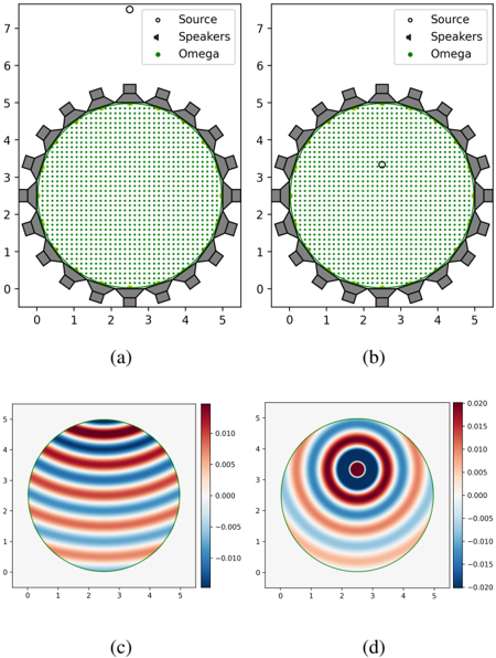
## Multi-Panel Chart: Wave Propagation Setups and Results ### Overview This image presents a 2x2 grid of plots, labeled (a) through (d), illustrating two distinct wave propagation setups and their corresponding simulated wave patterns within a circular domain. The top row (a, b) depicts the spatial arrangement of a "Source" and "Speakers" relative to a domain labeled "Omega". The bottom row (c, d) displays heatmaps of wave amplitudes within the "Omega" domain, corresponding to the setups above them. ### Components/Axes All four subplots share similar Cartesian coordinate systems. - **X-axis:** Ranges from 0 to 5, with major ticks at 0, 1, 2, 3, 4, 5. No explicit label is provided for the X-axis. - **Y-axis:** * For subplots (a) and (b): Ranges from 0 to 7, with major ticks at 0, 1, 2, 3, 4, 5, 6, 7. No explicit label is provided for the Y-axis. * For subplots (c) and (d): Ranges from 0 to 5, with major ticks at 0, 1, 2, 3, 4, 5. No explicit label is provided for the Y-axis. **Legend (Common to subplots (a) and (b), located top-right):** - `o` **Source**: Represented by a white circle with a black outline. - `▲` **Speakers**: Represented by a solid black upward-pointing triangle. - `•` **Omega**: Represented by a solid green circle. **Color Bars (Specific to subplots (c) and (d), located on the right side of each plot):** - **Subplot (c) Color Bar:** * Range: -0.010 to 0.010. * Major ticks: -0.010, -0.005, 0.000, 0.005, 0.010. * Color gradient: Deep blue at -0.010, transitioning through light blue, white (around 0.000), light red, to deep red at 0.010. - **Subplot (d) Color Bar:** * Range: -0.020 to 0.020. * Major ticks: -0.020, -0.015, -0.010, -0.005, 0.000, 0.005, 0.010, 0.015, 0.020. * Color gradient: Deep blue at -0.020, transitioning through light blue, white (around 0.000), light red, to deep red at 0.020. ### Detailed Analysis **Subplot (a): Setup with External Source** - **Type:** Diagram/Scatter Plot. - **Main Elements:** * A large grey gear-like structure with 20 teeth is centrally positioned, spanning approximately x-coordinates 0 to 5 and y-coordinates 0 to 5. Its center is roughly at (2.5, 2.5). * Inside the gear, a circular region, outlined in green, is densely filled with small green dots. This region represents "Omega" as per the legend. The "Omega" circle is centered at approximately (2.5, 2.5) with a radius of about 2.5 units. * Twenty black triangles, representing "Speakers", are arranged in a circle along the inner circumference of the gear structure, precisely on the green outline of the "Omega" domain. * A single white circle with a black outline, representing the "Source", is located significantly above the "Omega" domain, at approximately coordinates (2.5, 7.5). - **Label:** (a) is positioned at the bottom-left of the subplot. **Subplot (b): Setup with Internal Source** - **Type:** Diagram/Scatter Plot. - **Main Elements:** * The grey gear-like structure, the green-outlined "Omega" domain filled with green dots, and the twenty black "Speakers" are identical in position and appearance to subplot (a). * The "Source" (white circle with black outline) is positioned *inside* the "Omega" domain, slightly above its center, at approximately coordinates (2.5, 3.4). - **Label:** (b) is positioned at the bottom-left of the subplot. **Subplot (c): Wave Pattern for External Source Setup** - **Type:** Heatmap/Contour Plot. - **Main Elements:** * A circular region, outlined in green, is displayed, matching the "Omega" domain from subplots (a) and (b) in size and position (centered at approximately (2.5, 2.5) with a radius of about 2.5 units). * **Trend:** The heatmap shows a pattern of approximately 5-6 horizontal, parallel bands of alternating red and blue colors, separated by white regions. The bands are more intense (deeper red/blue) towards the top and bottom edges of the circle and fade towards the horizontal center line (y=2.5) where the colors are lighter or white. The pattern suggests a standing wave or a plane wave propagating vertically. * **Values:** The color bar indicates values ranging from -0.010 (deep blue) to 0.010 (deep red), with white representing values near 0.000. - **Label:** (c) is positioned at the bottom-left of the subplot. **Subplot (d): Wave Pattern for Internal Source Setup** - **Type:** Heatmap/Contour Plot. - **Main Elements:** * A circular region, outlined in green, is displayed, matching the "Omega" domain from subplots (a) and (b) in size and position (centered at approximately (2.5, 2.5) with a radius of about 2.5 units). * **Trend:** The heatmap displays a pattern of concentric rings of alternating red and blue colors, separated by white regions. The center of these rings is located at approximately (2.5, 3.4), which corresponds precisely to the "Source" location in subplot (b). The intensity (color saturation) is highest at the center (deep red) and in the outer rings, decreasing towards the white rings. This pattern is characteristic of a radially propagating wave originating from a point source. * **Values:** The color bar indicates values ranging from -0.020 (deep blue) to 0.020 (deep red), with white representing values near 0.000. The maximum amplitude in this plot is twice that of subplot (c). - **Label:** (d) is positioned at the bottom-left of the subplot. ### Key Observations - Subplots (a) and (b) illustrate two different source configurations for wave generation within the "Omega" domain, which is consistently a circular region surrounded by "Speakers" and a gear-like boundary. - Subplot (a) places the "Source" externally, high above the "Omega" domain. - Subplot (b) places the "Source" internally, within the "Omega" domain, slightly off-center. - Subplot (c) shows a wave pattern with horizontal bands, suggesting a wave field influenced by an external or distant source, possibly generating a plane-wave-like behavior or a specific mode. - Subplot (d) shows a wave pattern with concentric rings originating from the internal source location depicted in subplot (b), characteristic of a point source radiating waves. - The maximum amplitude of the wave field in (d) (0.020) is twice that in (c) (0.010), suggesting a stronger or differently scaled wave generation for the internal source case. - The "Speakers" are consistently positioned on the boundary of the "Omega" domain in both setups (a) and (b), implying they might be used to control or measure the wave field at the boundary. ### Interpretation The image effectively demonstrates the impact of source location on wave propagation patterns within a confined circular domain. The "Omega" domain, filled with green dots, likely represents the computational or physical space where the wave equation is solved or observed. The "Speakers" on the boundary suggest an active control or measurement system, possibly for acoustic or electromagnetic waves, where the gear-like structure might represent a physical enclosure or an array of transducers. Subplots (a) and (c) together suggest a scenario where an external "Source" (perhaps a distant plane wave source or a source whose effect is shaped by the "Speakers") generates a wave field that manifests as horizontal standing waves or modes within the "Omega" domain. The horizontal banding implies a dominant directionality or boundary condition effect. Conversely, subplots (b) and (d) illustrate a classic point-source radiation scenario. When the "Source" is placed directly inside the "Omega" domain, the resulting wave pattern (d) clearly shows circular wavefronts emanating from that source. The higher amplitude in (d) compared to (c) could indicate a more direct coupling of energy from the internal source to the domain, or simply a different scaling factor in the simulation/measurement. The consistent presence of the "Speakers" on the boundary of "Omega" in both setups implies their role is independent of the source's primary location (internal vs. external). They could be acting as sensors, actuators for active noise control, or simply defining the boundary conditions for the wave propagation. The overall presentation suggests a study of wave phenomena in a bounded region, exploring different excitation methods and their resulting field distributions.