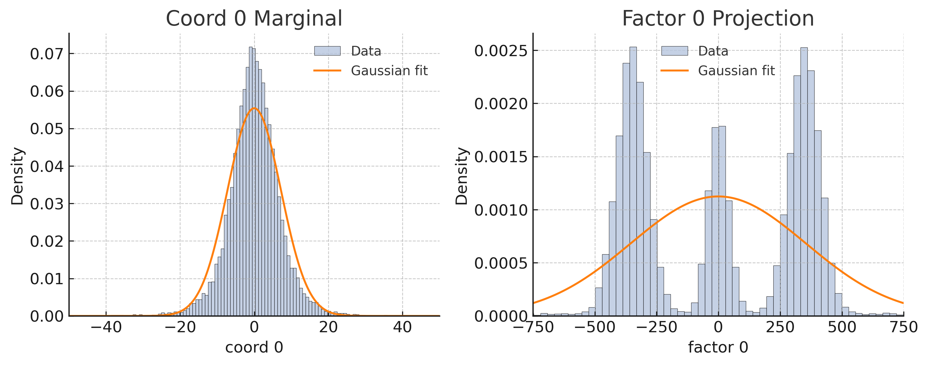
\n ## Histograms: Coordinate and Factor Projections ### Overview The image presents two histograms, side-by-side. The left histogram displays the marginal distribution of "Coord 0", while the right histogram shows the projection onto "Factor 0". Both histograms are overlaid with a Gaussian fit, indicated by a solid orange line. The histograms are designed to visualize the distribution of data along these two dimensions. ### Components/Axes **Left Histogram (Coord 0 Marginal):** * **Title:** "Coord 0 Marginal" (top-center) * **X-axis Label:** "coord 0" (bottom-center) - Scale ranges approximately from -40 to 40. * **Y-axis Label:** "Density" (left-center) - Scale ranges approximately from 0.00 to 0.07. * **Legend:** Located in the top-right corner. * "Data" - Represented by grey bars. * "Gaussian fit" - Represented by an orange line. **Right Histogram (Factor 0 Projection):** * **Title:** "Factor 0 Projection" (top-center) * **X-axis Label:** "factor 0" (bottom-center) - Scale ranges approximately from -750 to 750. * **Y-axis Label:** "Density" (left-center) - Scale ranges approximately from 0.000 to 0.0025. * **Legend:** Located in the top-right corner. * "Data" - Represented by grey bars. * "Gaussian fit" - Represented by an orange line. ### Detailed Analysis or Content Details **Left Histogram (Coord 0 Marginal):** The histogram shows a roughly symmetrical distribution centered around 0. The data is concentrated between -20 and 20. * **Data (Grey Bars):** The highest density occurs around coord 0, with a value of approximately 0.065. Density decreases as you move away from 0 in either direction. * **Gaussian Fit (Orange Line):** The Gaussian fit closely follows the shape of the data, peaking at approximately coord 0. The curve extends beyond the data, indicating the fitted distribution. **Right Histogram (Factor 0 Projection):** This histogram displays a bimodal distribution, with peaks around -250 and 250. * **Data (Grey Bars):** There are two prominent peaks. The peak on the left is around -250 with a density of approximately 0.0023. The peak on the right is around 250 with a density of approximately 0.0022. There are smaller peaks around -500 and 500 with densities of approximately 0.0005. * **Gaussian Fit (Orange Line):** The Gaussian fit attempts to approximate the bimodal distribution, but it doesn't capture the distinct peaks as accurately as it did for the first histogram. The curve shows a broad peak around 0, with lower values at the extremes. ### Key Observations * The "Coord 0" distribution is unimodal and centered around zero. * The "Factor 0" distribution is bimodal, suggesting two distinct clusters of data along this factor. * The Gaussian fit is a better representation of the "Coord 0" distribution than the "Factor 0" distribution. * The scale of the Y-axis differs significantly between the two histograms, reflecting the different densities of the data. ### Interpretation The data suggests that "Coord 0" represents a single, central tendency in the data, while "Factor 0" represents two distinct groupings or modes. The bimodal distribution of "Factor 0" could indicate the presence of two underlying populations or processes contributing to the data. The Gaussian fit for "Coord 0" implies that the data along this coordinate is well-approximated by a normal distribution. The poorer fit for "Factor 0" suggests that a Gaussian distribution is not an appropriate model for this dimension, likely due to the bimodal nature of the data. The difference in scales between the two histograms indicates that the data is more concentrated around the mean in "Coord 0" than in "Factor 0". This could be due to the nature of the variables themselves or the way the data was generated.