## Histograms: Coord 0 Marginal and Factor 0 Projection
### Overview
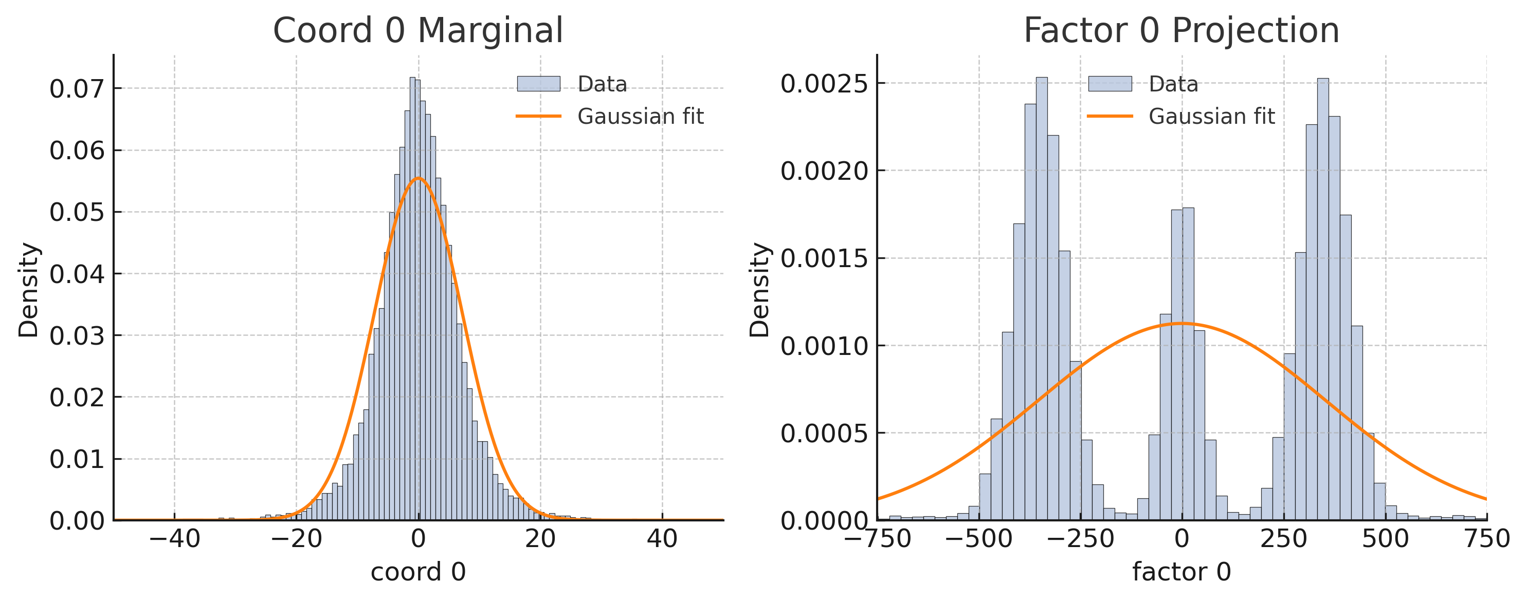
The image contains two side-by-side histograms. The left chart is titled "Coord 0 Marginal," and the right is titled "Factor 0 Projection." Both histograms display data distributions with overlaid Gaussian fit curves. The left histogram has a narrower range and a single peak, while the right histogram has a wider range and two distinct peaks.
### Components/Axes
- **Left Chart ("Coord 0 Marginal")**:
- **X-axis**: "coord 0" (range: -40 to 40, labeled in increments of 20).
- **Y-axis**: "Density" (range: 0.00 to 0.07, labeled in increments of 0.01).
- **Legend**: "Data" (gray bars) and "Gaussian fit" (orange line).
- **Right Chart ("Factor 0 Projection")**:
- **X-axis**: "factor 0" (range: -750 to 750, labeled in increments of 250).
- **Y-axis**: "Density" (range: 0.0000 to 0.0025, labeled in increments of 0.0005).
- **Legend**: "Data" (gray bars) and "Gaussian fit" (orange line).
### Detailed Analysis
- **Left Chart**:
- The histogram shows a bell-shaped distribution centered near 0.
- The Gaussian fit (orange line) closely matches the data, peaking at approximately 0.055 density.
- The data bars (gray) are tallest at 0, with density decreasing symmetrically toward -40 and 40.
- **Right Chart**:
- The histogram has two prominent peaks: one near -250 and another near 250.
- The Gaussian fit (orange line) is a single peak centered at 0, with a maximum density of ~0.0018.
- The data bars (gray) show higher density at -250 and 250 compared to the Gaussian fit, indicating a bimodal distribution.
### Key Observations
1. **Left Chart**: The Gaussian fit aligns well with the data, suggesting a normal distribution.
2. **Right Chart**: The Gaussian fit does not match the bimodal data, implying the fit may be inappropriate for this distribution.
3. **Density Scales**: The left chart’s density peaks at ~0.06, while the right chart’s peaks are ~0.002, indicating vastly different scales.
### Interpretation
- The left chart demonstrates a unimodal, symmetric distribution (likely a single variable’s marginal distribution).
- The right chart reveals a bimodal distribution (two clusters at -250 and 250), but the Gaussian fit assumes a single peak, which may misrepresent the data. This discrepancy could indicate:
- A need for a different model (e.g., mixture of Gaussians) for the right chart.
- Potential issues with data preprocessing or factor projection methodology.
- The stark difference in density scales between the two charts highlights the importance of context when comparing distributions.
## [Chart/Diagram Type]: Histograms
### Overview
Two histograms compare the distribution of "Coord 0" and "Factor 0" variables, with Gaussian fit curves overlaid.
### Components/Axes
- **Left Chart**:
- **X-axis**: "coord 0" (-40 to 40).
- **Y-axis**: "Density" (0.00 to 0.07).
- **Legend**: "Data" (gray), "Gaussian fit" (orange).
- **Right Chart**:
- **X-axis**: "factor 0" (-750 to 750).
- **Y-axis**: "Density" (0.0000 to 0.0025).
- **Legend**: "Data" (gray), "Gaussian fit" (orange).
### Detailed Analysis
- **Left Chart**:
- Data peaks at 0 with density ~0.06.
- Gaussian fit peaks at ~0.055, closely matching the data.
- **Right Chart**:
- Data peaks at -250 and 250 with density ~0.002.
- Gaussian fit peaks at 0 with density ~0.0018, misaligning with the bimodal data.
### Key Observations
- The left chart’s Gaussian fit is accurate for a normal distribution.
- The right chart’s Gaussian fit fails to capture the bimodal structure, suggesting model mismatch.
### Interpretation
The histograms highlight the importance of selecting appropriate statistical models. While the left chart’s Gaussian fit is valid, the right chart’s bimodal data requires a more complex model. This could impact downstream analyses, such as clustering or regression, if the factor projection is used without accounting for its multimodality.