\n
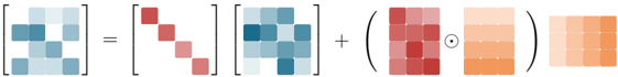
## Heatmaps: Matrix Decomposition Illustration
### Overview
The image depicts a visual representation of matrix decomposition, specifically illustrating how a matrix can be approximated by the sum of two lower-rank matrices. It consists of five heatmaps arranged horizontally, connected by mathematical symbols. The first heatmap is equated to the sum of the second and third heatmaps, which are then further decomposed into a product of two heatmaps enclosed in parentheses.
### Components/Axes
There are no explicit axes labels or legends present in the image. The heatmaps themselves represent matrices, with color intensity indicating the magnitude of the values within the matrix. Each heatmap is a 5x5 grid. The symbols "=", "+", and "()" are mathematical operators indicating equality, addition, and multiplication, respectively. A circled dot "⊙" is present, indicating element-wise multiplication.
### Detailed Analysis or Content Details
Let's analyze each heatmap individually, describing the color distribution and approximate values based on the color scale. The color scale appears to range from a deep blue (low value) to a bright red (high value), passing through shades of teal and orange.
**Heatmap 1 (Leftmost):**
This heatmap shows a generally cool color scheme, with predominantly blue and teal shades. There are a few warmer areas (orange) in the bottom-right corner and a small patch in the top-left.
* Top-left: ~0.2 (light blue)
* Top-right: ~0.3 (light blue)
* Center: ~0.4 (teal)
* Bottom-left: ~0.5 (teal)
* Bottom-right: ~0.7 (orange)
**Heatmap 2 (Second from Left):**
This heatmap is dominated by red and orange shades, indicating higher values.
* Top-left: ~0.8 (red)
* Top-right: ~0.2 (light blue)
* Center: ~0.3 (light blue)
* Bottom-left: ~0.7 (orange)
* Bottom-right: ~0.9 (red)
**Heatmap 3 (Middle):**
This heatmap is a mix of blue and teal shades, similar to the first heatmap, but with a slightly different distribution.
* Top-left: ~0.3 (light blue)
* Top-right: ~0.5 (teal)
* Center: ~0.2 (light blue)
* Bottom-left: ~0.4 (teal)
* Bottom-right: ~0.6 (teal)
**Heatmap 4 (Fourth from Left - Left Parenthesis):**
This heatmap is predominantly red and orange, with a few cooler shades.
* Top-left: ~0.9 (red)
* Top-right: ~0.6 (orange)
* Center: ~0.4 (teal)
* Bottom-left: ~0.7 (orange)
* Bottom-right: ~0.8 (red)
**Heatmap 5 (Rightmost - Right Parenthesis):**
This heatmap is mostly orange and red, with a gradient from left to right.
* Top-left: ~0.6 (orange)
* Top-right: ~0.9 (red)
* Center: ~0.7 (orange)
* Bottom-left: ~0.8 (red)
* Bottom-right: ~0.9 (red)
### Key Observations
The equation visually demonstrates that the first heatmap can be approximated by adding the second and third heatmaps. The decomposition further shows that the second and third heatmaps can be obtained by element-wise multiplication of the fourth and fifth heatmaps. The circled dot "⊙" confirms this is element-wise multiplication. The color distributions suggest that the first heatmap is a combination of the patterns present in the second and third heatmaps.
### Interpretation
This image illustrates a fundamental concept in linear algebra: matrix decomposition. Specifically, it demonstrates how a matrix can be broken down into simpler, lower-rank matrices. This is a common technique used in dimensionality reduction, data compression, and other applications. The visual representation using heatmaps effectively conveys the idea that the original matrix can be reconstructed by combining the information contained in the decomposed matrices. The use of color intensity to represent values makes it easy to see how the different matrices contribute to the overall structure of the original matrix. The element-wise multiplication suggests a form of factorization, where the original matrix is represented as a product of two matrices with specific properties. This is a simplified illustration, but it captures the essence of matrix decomposition and its potential applications.