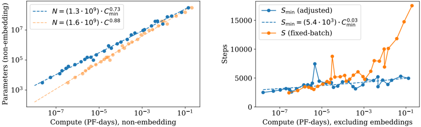
## Chart: Parameter Scaling vs. Compute ### Overview The image presents two scatter plots comparing compute (measured in PF-days) against parameters (non-embedding) and steps, respectively. The left plot shows the relationship between compute and the number of parameters, while the right plot shows the relationship between compute and the number of steps. Both plots use a log-log scale for the x-axis (Compute) and a log scale for the y-axis (Parameters or Steps). ### Components/Axes **Left Plot:** * **X-axis:** Compute (PF-days), non-embedding. Logarithmic scale from approximately 10^-7 to 10^-1. * **Y-axis:** Parameters (non-embedding). Logarithmic scale from 10^3 to 10^7. * **Data Series 1 (Blue):** `N = (1.3 * 10^9) * C_min^0.73` (dashed line) * **Data Series 2 (Orange):** `N = (1.6 * 10^9) * C_min^0.88` (dashed line) **Right Plot:** * **X-axis:** Compute (PF-days), excluding embeddings. Logarithmic scale from approximately 10^-7 to 10^-1. * **Y-axis:** Steps. Linear scale from 0 to 15000. * **Data Series 1 (Blue):** `S_min (adjusted)` (solid line with circular markers) * **Data Series 2 (Blue):** `S_min = (5.4 * 10^3) * C_min^0.03` (dashed line) * **Data Series 3 (Orange):** `S (fixed-batch)` (solid line with circular markers) ### Detailed Analysis **Left Plot (Parameters vs. Compute):** * **Blue Data Series:** The blue dashed line represents the equation `N = (1.3 * 10^9) * C_min^0.73`. The data points cluster closely around this line, indicating a strong relationship between compute and the number of parameters. As compute increases, the number of parameters also increases. * At Compute = 10^-7, Parameters ≈ 2000 * At Compute = 10^-1, Parameters ≈ 5 * 10^6 * **Orange Data Series:** The orange dashed line represents the equation `N = (1.6 * 10^9) * C_min^0.88`. The data points cluster closely around this line, indicating a strong relationship between compute and the number of parameters. As compute increases, the number of parameters also increases. The orange line is generally below the blue line. * At Compute = 10^-7, Parameters ≈ 1000 * At Compute = 10^-1, Parameters ≈ 3 * 10^6 **Right Plot (Steps vs. Compute):** * **Blue Data Series (Adjusted):** The blue solid line with circular markers represents `S_min (adjusted)`. The number of steps increases slightly with compute, but the relationship is not as clear as in the left plot. There is more variance in the data. * At Compute = 10^-7, Steps ≈ 2000 * At Compute = 10^-3, Steps ≈ 4000 * At Compute = 10^-2, Steps ≈ 3000 * At Compute = 10^-1, Steps ≈ 4000 * **Blue Data Series (Equation):** The blue dashed line represents the equation `S_min = (5.4 * 10^3) * C_min^0.03`. This line provides a smoothed representation of the relationship between compute and steps. * At Compute = 10^-7, Steps ≈ 3000 * At Compute = 10^-1, Steps ≈ 3500 * **Orange Data Series (Fixed-Batch):** The orange solid line with circular markers represents `S (fixed-batch)`. The number of steps increases significantly with compute, especially at higher compute values. The relationship is more pronounced than the adjusted steps. * At Compute = 10^-7, Steps ≈ 2000 * At Compute = 10^-3, Steps ≈ 3000 * At Compute = 10^-2, Steps ≈ 5000 * At Compute = 10^-1, Steps ≈ 15000 ### Key Observations * The left plot shows a strong positive correlation between compute and the number of parameters. * The right plot shows a weaker correlation between compute and the number of steps, especially for the adjusted steps. The fixed-batch steps show a more pronounced increase with compute. * The equations provided in the legends appear to be fitted models representing the relationships between the variables. ### Interpretation The plots suggest that increasing compute leads to a significant increase in the number of parameters in the non-embedding layers of the model. The relationship between compute and the number of steps is more complex. The adjusted steps show a relatively flat trend, while the fixed-batch steps show a more significant increase with compute, suggesting that the batch size influences the number of steps required. The difference between the adjusted and fixed-batch steps could be due to different optimization strategies or hyperparameter settings. The equations provided offer a quantitative way to estimate the number of parameters or steps given a certain amount of compute.

## Chart: Scaling of Parameters and Steps with Compute ### Overview The image presents two charts side-by-side, both examining the relationship between compute (measured in PF-days) and either the number of parameters (left chart) or the number of steps (right chart). Both charts display data for different configurations, indicated by different colored lines and associated equations. The left chart focuses on parameter scaling, while the right chart focuses on step scaling. ### Components/Axes **Left Chart:** * **X-axis:** Compute (PF-days), non-embedding. Scale is logarithmic, ranging from approximately 10^-7 to 10^-1. * **Y-axis:** Parameters (non-embedding). Scale is logarithmic, ranging from approximately 10³ to 10⁵. * **Lines/Legends:** * Blue dashed line: N = (1.3 * 10⁹) * C_min^0.73 * Orange dashed line: N = (1.6 * 10⁹) * C_min^0.88 **Right Chart:** * **X-axis:** Compute (PF-days), excluding embeddings. Scale is logarithmic, ranging from approximately 10^-7 to 10^-1. * **Y-axis:** Steps. Scale is linear, ranging from 0 to 15000. * **Lines/Legends:** * Blue dashed line: S_min (adjusted) = (5.4 * 10³) * C_min^0.03 * Orange solid line: S (fixed-batch) ### Detailed Analysis or Content Details **Left Chart (Parameters vs. Compute):** * The blue line (N = (1.3 * 10⁹) * C_min^0.73) starts at approximately 10^3.2 parameters at 10^-7 PF-days and rises to approximately 10^4.8 parameters at 10^-1 PF-days. The line exhibits a generally upward trend, with a slight concavity. * The orange line (N = (1.6 * 10⁹) * C_min^0.88) starts at approximately 10³ parameters at 10^-7 PF-days and rises to approximately 10⁵ parameters at 10^-1 PF-days. This line also exhibits an upward trend, but is steeper than the blue line, especially at higher compute values. **Right Chart (Steps vs. Compute):** * The blue line (S_min (adjusted) = (5.4 * 10³) * C_min^0.03) starts at approximately 2000 steps at 10^-7 PF-days, dips to around 1500 steps at 10^-5 PF-days, then rises to approximately 4000 steps at 10^-1 PF-days. The line is relatively flat initially, then shows some fluctuations before a slight increase. * The orange line (S (fixed-batch)) starts at approximately 2500 steps at 10^-7 PF-days, remains relatively stable until approximately 10^-3 PF-days, then increases sharply to approximately 14000 steps at 10^-1 PF-days. This line shows a much more pronounced increase in steps at higher compute values. ### Key Observations * Both charts demonstrate a positive correlation between compute and the respective metrics (parameters and steps). * The parameter scaling (left chart) shows that the orange configuration (higher coefficient) requires more parameters than the blue configuration for a given compute value. * The step scaling (right chart) shows a significant divergence between the adjusted (blue) and fixed-batch (orange) approaches at higher compute values, with the fixed-batch approach requiring substantially more steps. * The adjusted step scaling (blue line, right chart) exhibits a dip in steps around 10^-5 PF-days, suggesting a potential optimization or efficiency gain at that compute level. ### Interpretation The data suggests that increasing compute leads to increased model size (parameters) and training effort (steps). The two parameter scaling curves (left chart) indicate different scaling efficiencies, with the orange curve representing a configuration that requires more parameters for a given compute budget. The right chart highlights the trade-offs between different step scaling strategies. The fixed-batch approach (orange line) becomes significantly more expensive in terms of steps as compute increases, while the adjusted approach (blue line) maintains a more moderate increase. The dip in the adjusted step scaling curve around 10^-5 PF-days could indicate a point where algorithmic optimizations become effective, reducing the number of steps needed for a given level of compute. The equations provided suggest that both parameters and steps scale with C_min to some power, indicating that the minimum compute unit plays a role in determining the overall resource requirements. The difference in exponents (0.73 vs 0.88 for parameters, and 0.03 for steps) suggests that parameters are more sensitive to changes in C_min than steps.

## Scatter Plot Charts: Scaling Laws for Neural Network Parameters and Training Steps ### Overview The image contains two side-by-side scatter plot charts on a white background. Both charts analyze relationships between computational resources (measured in PF-days) and model characteristics (parameters or training steps) on logarithmic scales. The charts appear to illustrate scaling laws, likely in the context of machine learning model training. ### Components/Axes **Left Chart:** * **Chart Type:** Scatter plot with logarithmic axes. * **X-axis:** Label: `Compute (PF-days), non-embedding`. Scale: Logarithmic, ranging from approximately `10^-8` to `10^-1`. * **Y-axis:** Label: `Parameters (non-embedding)`. Scale: Logarithmic, ranging from `10^2` to `10^8`. * **Legend (Top-Left):** * Blue dashed line: `N = (1.3 * 10^9) * C_min^0.73` * Orange dashed line: `N = (1.6 * 10^9) * C_min^0.88` * **Data Series:** * Blue dots: Represent data points corresponding to the blue dashed line model. * Orange dots: Represent data points corresponding to the orange dashed line model. **Right Chart:** * **Chart Type:** Scatter plot with one logarithmic axis. * **X-axis:** Label: `Compute (PF-days), excluding embeddings`. Scale: Logarithmic, ranging from approximately `10^-8` to `10^-1`. * **Y-axis:** Label: `Steps`. Scale: Linear, ranging from `0` to `15000`. * **Legend (Top-Left):** * Blue line with circle markers: `S_min (adjusted)` * Blue dashed line: `S_min = (5.4 * 10^3) * C_min^0.03` * Orange line with circle markers: `S (fixed-batch)` * **Data Series:** * Blue line with markers (`S_min (adjusted)`): Shows a generally increasing trend with significant local variability and spikes. * Orange line with markers (`S (fixed-batch)`): Shows a clear, steeply increasing trend, especially at higher compute values. ### Detailed Analysis **Left Chart (Parameters vs. Compute):** * **Trend Verification:** Both data series show a strong, positive, linear correlation on the log-log plot, indicating a power-law relationship. The blue series has a slightly shallower slope than the orange series. * **Data Points & Equations:** * The blue dots closely follow the trend line defined by the equation `N = (1.3 * 10^9) * C_min^0.73`. The exponent `0.73` indicates that model parameter count scales with compute to the power of 0.73 for this series. * The orange dots closely follow the trend line defined by the equation `N = (1.6 * 10^9) * C_min^0.88`. The exponent `0.88` indicates a stronger scaling relationship for this series. * At the lowest compute (`~10^-8` PF-days), the orange series predicts slightly fewer parameters than the blue series. Due to its steeper slope, the orange series surpasses the blue series at approximately `10^-5` PF-days and predicts significantly more parameters at the highest compute (`~10^-1` PF-days). **Right Chart (Steps vs. Compute):** * **Trend Verification:** The `S (fixed-batch)` (orange) series shows a clear, accelerating upward trend. The `S_min (adjusted)` (blue) series shows a very shallow upward trend with high variance. * **Data Points & Equations:** * The blue dashed trend line for `S_min` is defined by `S_min = (5.4 * 10^3) * C_min^0.03`. The very small exponent (`0.03`) suggests the optimal number of training steps (`S_min`) is nearly independent of the total compute budget (`C_min`), increasing only marginally. * The `S_min (adjusted)` (blue line) data points scatter around this shallow trend line but exhibit notable spikes (e.g., near `10^-5` and `10^-4` PF-days). * The `S (fixed-batch)` (orange line) data points start near the `S_min` values at low compute but diverge dramatically upward as compute increases. At `~10^-1` PF-days, the fixed-batch steps (`~17,000`) are more than three times the adjusted optimal steps (`~5,000`). ### Key Observations 1. **Power-Law Scaling:** The left chart confirms a power-law relationship between model size (parameters) and compute, a fundamental observation in neural scaling laws. 2. **Divergent Step Scaling:** The right chart reveals a critical insight: while the *optimal* training steps (`S_min`) scale very weakly with compute (exponent `0.03`), using a *fixed batch size* (`S (fixed-batch)`) forces a much stronger increase in steps (visually, an exponent much greater than 0.03). 3. **Efficiency Gap:** The growing vertical gap between the orange and blue lines in the right chart represents an efficiency loss. As more compute is allocated, a fixed-batch strategy requires disproportionately more training steps compared to an optimally adjusted strategy. 4. **Variability in Optimal Steps:** The spikes in the `S_min (adjusted)` data suggest that the optimal number of steps may be sensitive to specific configurations or exhibit non-monotonic behavior at certain compute scales. ### Interpretation These charts together illustrate a core tension in scaling neural networks. The left chart shows the predictable, favorable scaling of model capacity with increased compute. However, the right chart exposes a crucial operational constraint: to fully utilize that increased compute for training a larger model, one cannot simply increase the batch size linearly. The `S_min` trend suggests that the optimal training duration (in steps) remains relatively constant, meaning the batch size must increase almost proportionally with the total compute budget to maintain efficiency. The `S (fixed-batch)` line demonstrates the consequence of failing to adjust the batch size: training becomes inefficient, requiring many more steps (and thus more time) to consume the same compute budget, likely leading to suboptimal model performance. The data argues for dynamic batch size scaling as a critical component of efficient large-scale model training. The near-zero exponent for `S_min` is a key quantitative finding, implying that for optimal efficiency, training step count should be held roughly constant as models and compute scale up, with batch size being the primary lever for utilizing additional resources.

## Scatter Plots: Compute vs. Parameters and Steps ### Overview The image contains two side-by-side scatter plots comparing computational efficiency metrics. The left plot shows the relationship between compute (PF-days) and parameters (non-embedding), while the right plot compares compute (excluding embeddings) to steps (training iterations). Both plots use logarithmic scales on the x-axis and linear scales on the y-axis. ### Components/Axes **Left Plot:** - **X-axis**: Compute (PF-days), non-embedding (log scale: 1e-7 to 1e-1) - **Y-axis**: Parameters (non-embedding) (log scale: 1e3 to 1e7) - **Legend**: - Blue dashed line: N = 1.3e9, C_min^0.73 - Orange dotted line: N = 1.6e9, C_min^0.88 **Right Plot:** - **X-axis**: Compute (PF-days), excluding embeddings (log scale: 1e-7 to 1e-1) - **Y-axis**: Steps (linear scale: 0 to 15,000) - **Legend**: - Blue solid circles: S_min (adjusted) - Blue dashed line: S_min = 5.4e3 * C_min^0.03 - Orange squares: S (fixed-batch) ### Detailed Analysis **Left Plot Trends:** 1. Both data series show a positive correlation between compute and parameters. 2. The orange series (N=1.6e9) has a steeper slope (C_min^0.88) compared to the blue series (C_min^0.73). 3. At 1e-3 PF-days, parameters reach ~1e6 for N=1.3e9 and ~1e6.5 for N=1.6e9. 4. At 1e-1 PF-days, parameters approach ~1e7 for both series. **Right Plot Trends:** 1. S_min (adjusted) (blue circles) remains relatively stable (~2,000-4,000 steps) across compute ranges. 2. S_min = 5.4e3 * C_min^0.03 (blue dashed) shows minor fluctuations but stays below 5,000 steps. 3. S (fixed-batch) (orange squares) exhibits exponential growth: - 1e-7 PF-days: ~1,000 steps - 1e-5 PF-days: ~5,000 steps - 1e-3 PF-days: ~10,000 steps - 1e-1 PF-days: ~15,000 steps ### Key Observations 1. **Non-embedding parameters** scale polynomially with compute, with higher N values yielding steeper growth. 2. **Fixed-batch steps** increase dramatically with compute, while adjusted S_min remains stable. 3. The orange series in the left plot (N=1.6e9) consistently outperforms the blue series (N=1.3e9) in parameter efficiency. 4. The right plot reveals a critical threshold: fixed-batch steps surge beyond 1e-3 PF-days, suggesting diminishing returns for larger compute budgets. ### Interpretation The data demonstrates fundamental trade-offs in model training: 1. **Parameter Efficiency**: Larger N values (1.6e9 vs. 1.3e9) achieve higher parameter counts per compute unit, but with diminishing returns (exponent 0.88 vs. 0.73). 2. **Step Efficiency**: Fixed-batch training becomes prohibitively expensive at scale, while adjusted S_min maintains stability through dynamic batch sizing. 3. **Compute Thresholds**: The right plot's exponential step growth beyond 1e-3 PF-days suggests a practical limit for fixed-batch training, while adjusted methods remain viable. These findings highlight the importance of adaptive training strategies (like S_min adjustment) for large-scale model training, particularly when compute resources exceed 1e-3 PF-days.