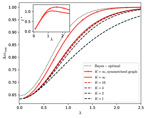
## Line Chart: Accuracy vs. Lambda for Different K Values ### Overview The image is a line chart showing the relationship between test accuracy (Acc_test) and a parameter lambda (λ) for different values of K. An inset plot shows the relationship between t* and lambda. The chart compares the performance of different models (characterized by K values) against a Bayes-optimal baseline. ### Components/Axes * **X-axis:** λ (lambda), ranging from 0.0 to 2.5 in increments of 0.5. * **Y-axis:** Acc_test (Test Accuracy), ranging from 0.65 to 1.00 in increments of 0.05. * **Legend (Bottom-Right):** * Black dotted line: Bayes - optimal * Red line with square markers: K = ∞, symmetrized graph * Red line: K = ∞ * Brown dashed line: K = 16 * Brown dash-dot line: K = 4 * Black dashed line: K = 2 * Black dash-dot line: K = 1 * **Inset Plot (Top-Left):** * X-axis: λ (lambda), ranging from 0 to 2 in increments of 1. * Y-axis: t*, ranging from 0.0 to 1.0 in increments of 0.5. * Red line: t* vs. lambda ### Detailed Analysis **Main Chart:** * **Bayes - optimal (Black dotted line):** Starts at approximately 0.64 at λ = 0, increases steadily, and approaches 1.00 as λ approaches 2.5. * λ = 0.0, Acc_test ≈ 0.64 * λ = 0.5, Acc_test ≈ 0.75 * λ = 1.0, Acc_test ≈ 0.85 * λ = 1.5, Acc_test ≈ 0.92 * λ = 2.0, Acc_test ≈ 0.97 * λ = 2.5, Acc_test ≈ 0.99 * **K = ∞, symmetrized graph (Red line with square markers):** Starts at approximately 0.64 at λ = 0, increases rapidly, peaks around λ = 1.5 at approximately 1.00, and then slightly decreases to approximately 0.99 as λ approaches 2.5. * λ = 0.0, Acc_test ≈ 0.64 * λ = 0.5, Acc_test ≈ 0.82 * λ = 1.0, Acc_test ≈ 0.96 * λ = 1.5, Acc_test ≈ 1.00 * λ = 2.0, Acc_test ≈ 0.99 * λ = 2.5, Acc_test ≈ 0.99 * **K = ∞ (Red line):** Starts at approximately 0.64 at λ = 0, increases rapidly, and approaches 0.98 as λ approaches 2.5. * λ = 0.0, Acc_test ≈ 0.64 * λ = 0.5, Acc_test ≈ 0.78 * λ = 1.0, Acc_test ≈ 0.90 * λ = 1.5, Acc_test ≈ 0.95 * λ = 2.0, Acc_test ≈ 0.97 * λ = 2.5, Acc_test ≈ 0.98 * **K = 16 (Brown dashed line):** Starts at approximately 0.64 at λ = 0, increases steadily, and approaches 0.95 as λ approaches 2.5. * λ = 0.0, Acc_test ≈ 0.64 * λ = 0.5, Acc_test ≈ 0.73 * λ = 1.0, Acc_test ≈ 0.83 * λ = 1.5, Acc_test ≈ 0.90 * λ = 2.0, Acc_test ≈ 0.93 * λ = 2.5, Acc_test ≈ 0.95 * **K = 4 (Brown dash-dot line):** Starts at approximately 0.64 at λ = 0, increases steadily, and approaches 0.90 as λ approaches 2.5. * λ = 0.0, Acc_test ≈ 0.64 * λ = 0.5, Acc_test ≈ 0.70 * λ = 1.0, Acc_test ≈ 0.78 * λ = 1.5, Acc_test ≈ 0.85 * λ = 2.0, Acc_test ≈ 0.88 * λ = 2.5, Acc_test ≈ 0.90 * **K = 2 (Black dashed line):** Starts at approximately 0.64 at λ = 0, increases steadily, and approaches 0.85 as λ approaches 2.5. * λ = 0.0, Acc_test ≈ 0.64 * λ = 0.5, Acc_test ≈ 0.68 * λ = 1.0, Acc_test ≈ 0.74 * λ = 1.5, Acc_test ≈ 0.80 * λ = 2.0, Acc_test ≈ 0.83 * λ = 2.5, Acc_test ≈ 0.85 * **K = 1 (Black dash-dot line):** Starts at approximately 0.63 at λ = 0, increases steadily, and approaches 0.80 as λ approaches 2.5. * λ = 0.0, Acc_test ≈ 0.63 * λ = 0.5, Acc_test ≈ 0.67 * λ = 1.0, Acc_test ≈ 0.72 * λ = 1.5, Acc_test ≈ 0.77 * λ = 2.0, Acc_test ≈ 0.79 * λ = 2.5, Acc_test ≈ 0.80 **Inset Plot:** * **t* vs. lambda (Red line):** Starts at approximately 0.2 at λ = 0, increases rapidly, peaks around λ = 1.5 at approximately 1.00, and then slightly decreases to approximately 0.98 as λ approaches 2. * λ = 0.0, t* ≈ 0.2 * λ = 0.5, t* ≈ 0.6 * λ = 1.0, t* ≈ 0.9 * λ = 1.5, t* ≈ 1.0 * λ = 2.0, t* ≈ 0.98 ### Key Observations * As λ increases, the test accuracy generally increases for all values of K. * Higher values of K generally lead to higher test accuracy. * The "K = ∞, symmetrized graph" model achieves the highest accuracy, peaking around λ = 1.5. * The Bayes-optimal model provides an upper bound on the achievable accuracy. * The inset plot shows that t* also increases with λ, peaking around λ = 1.5. ### Interpretation The chart demonstrates the impact of the parameter λ and the value of K on the test accuracy of a model. The "K = ∞, symmetrized graph" model performs best, suggesting that symmetrizing the graph and using a large K value can significantly improve accuracy. The Bayes-optimal line serves as a benchmark, showing the theoretical maximum accuracy achievable. The inset plot suggests a relationship between λ and t*, where t* also peaks around λ = 1.5, potentially indicating an optimal operating point for the model. The data suggests that increasing λ generally improves accuracy, but the effect diminishes as λ becomes larger. The choice of K also plays a crucial role, with higher K values generally leading to better performance.

## Chart: Test Accuracy vs. Lambda ### Overview The image presents a line chart illustrating the relationship between test accuracy (Acc_test) and a parameter lambda (λ) for different values of K. An inset chart shows a separate relationship between a value 'x*' and lambda. The chart compares the performance of different models or configurations, likely in a machine learning context. ### Components/Axes * **X-axis:** Lambda (λ), ranging from approximately 0.0 to 2.5. * **Y-axis:** Test Accuracy (Acc_test), ranging from approximately 0.65 to 1.00. * **Legend:** Located in the top-right corner, identifies the different lines: * Bayes – optimal (dotted black line) * K = ∞, symmetrized graph (solid red line) * K = ∞ (solid red line) * K = 16 (dashed red line) * K = 4 (dashed brown line) * K = 2 (dashed gray line) * K = 1 (dashed black line) * **Inset Chart:** Located in the top-left corner, shows a plot of 'x*' versus lambda (λ), ranging from approximately 0.0 to 2.0 for lambda and 0.0 to 1.0 for x*. ### Detailed Analysis The main chart displays several curves representing different values of K. * **Bayes – optimal (dotted black line):** This line starts at approximately 0.66 at λ = 0.0, increases rapidly, and reaches approximately 0.98 at λ = 1.0, then plateaus. * **K = ∞, symmetrized graph (solid red line):** This line starts at approximately 0.66 at λ = 0.0, increases more slowly than the Bayes line, reaches approximately 0.99 at λ = 1.5, and plateaus. * **K = ∞ (solid red line):** This line is nearly identical to the "K = ∞, symmetrized graph" line, starting at approximately 0.66 at λ = 0.0, increasing slowly, and reaching approximately 0.99 at λ = 1.5, then plateaus. * **K = 16 (dashed red line):** This line starts at approximately 0.66 at λ = 0.0, increases at a moderate rate, reaches approximately 0.95 at λ = 1.5, and plateaus. * **K = 4 (dashed brown line):** This line starts at approximately 0.66 at λ = 0.0, increases at a slower rate than K=16, reaches approximately 0.85 at λ = 1.5, and plateaus. * **K = 2 (dashed gray line):** This line starts at approximately 0.66 at λ = 0.0, increases slowly, reaches approximately 0.75 at λ = 1.5, and plateaus. * **K = 1 (dashed black line):** This line starts at approximately 0.66 at λ = 0.0, increases slowly, reaches approximately 0.70 at λ = 1.5, and plateaus. The inset chart shows a single curve. * **Inset Chart:** The curve starts at approximately 0.4 at λ = 0.0, increases to a peak of approximately 1.0 at λ = 1.0, and then decreases to approximately 0.7 at λ = 2.0. ### Key Observations * The Bayes – optimal line consistently outperforms all other configurations across the range of λ. * As K increases, the test accuracy generally increases, with K = ∞ providing the best performance among the K-based models. * The inset chart shows a non-monotonic relationship between 'x*' and λ, peaking at λ = 1.0. * All lines start at the same accuracy level (approximately 0.66) when λ = 0.0. ### Interpretation The chart demonstrates the impact of the parameter K on the test accuracy of a model as a function of lambda. The "Bayes – optimal" line represents a theoretical upper bound on performance. The results suggest that increasing K generally improves performance, approaching the optimal Bayes solution as K approaches infinity. The inset chart likely represents a related parameter or metric that influences the overall model behavior, exhibiting a peak performance at a specific value of lambda. The fact that all lines start at the same accuracy suggests that the initial performance is independent of K, but the subsequent improvement is heavily influenced by it. The plateauing of the lines at higher lambda values indicates that the model reaches a saturation point where further increases in lambda do not lead to significant improvements in accuracy. This could be due to overfitting or other limitations of the model.

## Line Graph with Inset: Test Accuracy vs. λ for Different K Values ### Overview The image displays a line graph plotting test accuracy (`Acc_test`) against a parameter `λ` (lambda). It compares the performance of a model under different conditions, primarily varying a parameter `K`. An inset graph in the top-left corner shows the relationship between an optimal parameter `t*` and `λ` for two specific cases. The overall trend shows accuracy improving with increasing `λ`, with different `K` values leading to distinct performance curves. ### Components/Axes **Main Chart:** * **X-axis:** Label is `λ`. Scale runs from 0.0 to 2.5, with major ticks at 0.0, 0.5, 1.0, 1.5, 2.0, 2.5. * **Y-axis:** Label is `Acc_test`. Scale runs from 0.65 to 1.00, with major ticks at 0.65, 0.70, 0.75, 0.80, 0.85, 0.90, 0.95, 1.00. * **Legend:** Located in the bottom-right quadrant. Contains seven entries: 1. `Bayes – optimal`: Dotted black line. 2. `K = ∞, symmetrized graph`: Solid red line. 3. `K = ∞`: Solid red line (visually identical in style to the symmetrized version, but represents a different data series). 4. `K = 16`: Dashed red line. 5. `K = 4`: Dashed red line. 6. `K = 2`: Dashed black line. 7. `K = 1`: Dashed black line. **Inset Chart (Top-Left Corner):** * **X-axis:** Label is `λ`. Scale runs from 0 to 2, with ticks at 0, 1, 2. * **Y-axis:** Label is `t*`. Scale runs from 0.0 to 1.0, with ticks at 0.0, 0.5, 1.0. * **Data Series:** Two solid red lines, corresponding to the `K = ∞` and `K = ∞, symmetrized graph` series from the main legend. ### Detailed Analysis **Main Chart Trends & Approximate Data Points:** * **Bayes-optimal (dotted black):** This line represents the theoretical upper bound. It starts at ~0.65 accuracy at λ=0, rises steeply, and asymptotically approaches 1.00 by λ≈2.0. * **K = ∞, symmetrized graph (solid red):** This is the highest-performing practical model. It starts near 0.63 at λ=0, follows a sigmoidal curve, and closely approaches the Bayes-optimal line, reaching ~0.99 by λ=2.5. * **K = ∞ (solid red):** Performs slightly below the symmetrized version. Starts near 0.63 at λ=0, follows a similar sigmoidal shape, and reaches ~0.98 by λ=2.5. * **K = 16 (dashed red):** Starts near 0.63 at λ=0. Its curve is below the K=∞ lines. It reaches ~0.97 by λ=2.5. * **K = 4 (dashed red):** Starts near 0.63 at λ=0. Its curve is below the K=16 line. It reaches ~0.96 by λ=2.5. * **K = 2 (dashed black):** Starts near 0.63 at λ=0. Its curve is below the K=4 line. It reaches ~0.95 by λ=2.5. * **K = 1 (dashed black):** This is the lowest-performing model. It starts near 0.63 at λ=0 and rises more slowly than all others, reaching only ~0.92 by λ=2.5. **Inset Chart Trends:** * The inset shows the optimal value of a parameter `t*` as a function of `λ` for the two `K=∞` cases. * Both red lines show `t*` increasing from 0 at λ=0, peaking at a value slightly above 1.0 around λ≈1.5, and then beginning to decrease as λ approaches 2. * The `K = ∞, symmetrized graph` line appears to have a slightly higher peak `t*` value than the standard `K = ∞` line. ### Key Observations 1. **Performance Hierarchy:** There is a clear and consistent performance hierarchy: Bayes-optimal > K=∞ (symmetrized) > K=∞ > K=16 > K=4 > K=2 > K=1. This order is maintained across the entire range of λ shown. 2. **Impact of K:** Increasing the parameter `K` monotonically improves test accuracy. The gap between consecutive `K` values (e.g., between K=1 and K=2, or K=4 and K=16) is significant at lower λ but narrows as λ increases and all models approach saturation. 3. **Sigmoidal Shape:** All accuracy curves exhibit a sigmoidal (S-shaped) growth pattern, indicating a phase of rapid improvement followed by diminishing returns. 4. **Asymptotic Behavior:** All models, even K=1, show accuracy improving with λ and trending towards an asymptote near 1.0, though the rate of convergence differs drastically. 5. **Inset Correlation:** The peak in `t*` around λ=1.5 in the inset corresponds to the region in the main chart where the accuracy curves for the high-K models begin to flatten significantly, suggesting `t*` may be a parameter governing the transition to the saturation regime. ### Interpretation This graph likely comes from a study on graph neural networks or semi-supervised learning, where `K` could represent the number of neighbors, message-passing steps, or a similar complexity parameter. `λ` is probably a regularization or noise parameter. The data demonstrates a fundamental trade-off: **model complexity (`K`) versus robustness to the parameter `λ`**. Simpler models (low `K`) are less effective overall and more sensitive to `λ`, showing slower accuracy gains. More complex models (high `K`, especially with symmetrization) achieve near-optimal performance much faster and are more robust, maintaining high accuracy across a wider range of `λ`. The "Bayes-optimal" line serves as a benchmark, showing the maximum achievable accuracy given the data. The fact that the `K=∞, symmetrized graph` model nearly matches it suggests that with sufficient complexity and the right inductive bias (symmetrization), the model can capture almost all predictable patterns in the data. The inset's `t*` parameter likely controls a threshold or temperature in the model; its non-monotonic relationship with `λ` indicates an optimal operating point that shifts with the data's noise or regularization level. The overall message is that investing in model complexity (`K`) and proper graph symmetrization yields substantial gains in both peak performance and robustness.

## Line Graph: Test Accuracy vs. Regularization Parameter (λ) ### Overview The graph depicts the relationship between the regularization parameter λ and test accuracy (Acc_test) for different model configurations. A secondary inset graph highlights the behavior near λ=0. The primary trend shows test accuracy increasing with λ up to a point before plateauing, with performance varying by model complexity (K). ### Components/Axes - **X-axis (λ)**: Regularization parameter ranging from 0.0 to 2.5. - **Y-axis (Acc_test)**: Test accuracy ranging from 0.65 to 1.00. - **Legend**: Located in the bottom-right corner, with six entries: - Dotted black: Bayes – optimal - Solid red: K = ∞, symmetrized graph - Dashed red: K = ∞ - Dashed brown: K = 16 - Dashed maroon: K = 4 - Dashed black: K = 2 - Solid black: K = 1 ### Detailed Analysis 1. **Bayes – optimal (dotted black line)**: - Remains consistently above all other lines across all λ values. - Peaks at λ ≈ 1.2 with Acc_test ≈ 0.99, then plateaus. - Spatial grounding: Topmost line, positioned centrally in the graph. 2. **K = ∞, symmetrized graph (solid red line)**: - Second-highest performance, closely tracking the Bayes-optimal line. - Peaks at λ ≈ 1.1 with Acc_test ≈ 0.985, then plateaus. - Spatial grounding: Directly below the Bayes-optimal line. 3. **K = ∞ (dashed red line)**: - Third-highest performance, slightly below the solid red line. - Peaks at λ ≈ 1.0 with Acc_test ≈ 0.98, then plateaus. - Spatial grounding: Below the solid red line, with dashed pattern. 4. **K = 16 (dashed brown line)**: - Peaks at λ ≈ 0.8 with Acc_test ≈ 0.95, then declines slightly. - Spatial grounding: Below K = ∞ lines, with a noticeable dip after λ=1. 5. **K = 4 (dashed maroon line)**: - Peaks at λ ≈ 0.6 with Acc_test ≈ 0.92, then declines. - Spatial grounding: Below K = 16, with a steeper decline post-λ=1. 6. **K = 2 (dashed black line)**: - Peaks at λ ≈ 0.4 with Acc_test ≈ 0.88, then declines. - Spatial grounding: Below K = 4, with a pronounced downward trend after λ=0.5. 7. **K = 1 (solid black line)**: - Lowest performance, peaks at λ ≈ 0.2 with Acc_test ≈ 0.85. - Spatial grounding: Bottommost line, with minimal improvement beyond λ=0.3. **Inset Graph**: - Zoomed-in view of the main graph’s lower-left region (λ=0 to 2, Acc_test=0.65 to 1.0). - Confirms the trend of increasing accuracy with λ up to λ=1, then plateauing. - Highlights the divergence between high-K and low-K models at small λ values. ### Key Observations 1. **Optimal λ**: All models achieve peak performance near λ=1, with Bayes-optimal and K=∞ configurations performing best. 2. **Model Complexity Trade-off**: Higher K values (e.g., K=∞) achieve higher accuracy but require larger λ to avoid overfitting. Lower K values (e.g., K=1) underperform but are less sensitive to λ. 3. **Performance Saturation**: Beyond λ=1.5, all models plateau, suggesting diminishing returns from increased regularization. 4. **Inset Confirmation**: The zoomed-in view validates the main trend, emphasizing the critical region near λ=0 where performance differences are most pronounced. ### Interpretation The graph demonstrates that model complexity (K) and regularization (λ) are interdependent factors in achieving optimal test accuracy. The Bayes-optimal configuration (dotted black line) represents the theoretical upper bound, while practical models (K=∞, K=16, etc.) approach this bound with appropriate λ tuning. The inset graph underscores that even small λ values significantly impact performance for low-K models, but higher-K models require larger λ to balance complexity and generalization. The plateau at λ>1.5 suggests that excessive regularization degrades performance, reinforcing the need for careful hyperparameter tuning. The spatial alignment of lines (e.g., K=∞ configurations clustering near the top) visually reinforces the trade-off between model capacity and regularization strength.