## Line Graph with Inset: Test Accuracy vs. λ for Different K Values
### Overview
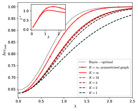
The image displays a line graph plotting test accuracy (`Acc_test`) against a parameter `λ` (lambda). It compares the performance of a model under different conditions, primarily varying a parameter `K`. An inset graph in the top-left corner shows the relationship between an optimal parameter `t*` and `λ` for two specific cases. The overall trend shows accuracy improving with increasing `λ`, with different `K` values leading to distinct performance curves.
### Components/Axes
**Main Chart:**
* **X-axis:** Label is `λ`. Scale runs from 0.0 to 2.5, with major ticks at 0.0, 0.5, 1.0, 1.5, 2.0, 2.5.
* **Y-axis:** Label is `Acc_test`. Scale runs from 0.65 to 1.00, with major ticks at 0.65, 0.70, 0.75, 0.80, 0.85, 0.90, 0.95, 1.00.
* **Legend:** Located in the bottom-right quadrant. Contains seven entries:
1. `Bayes – optimal`: Dotted black line.
2. `K = ∞, symmetrized graph`: Solid red line.
3. `K = ∞`: Solid red line (visually identical in style to the symmetrized version, but represents a different data series).
4. `K = 16`: Dashed red line.
5. `K = 4`: Dashed red line.
6. `K = 2`: Dashed black line.
7. `K = 1`: Dashed black line.
**Inset Chart (Top-Left Corner):**
* **X-axis:** Label is `λ`. Scale runs from 0 to 2, with ticks at 0, 1, 2.
* **Y-axis:** Label is `t*`. Scale runs from 0.0 to 1.0, with ticks at 0.0, 0.5, 1.0.
* **Data Series:** Two solid red lines, corresponding to the `K = ∞` and `K = ∞, symmetrized graph` series from the main legend.
### Detailed Analysis
**Main Chart Trends & Approximate Data Points:**
* **Bayes-optimal (dotted black):** This line represents the theoretical upper bound. It starts at ~0.65 accuracy at λ=0, rises steeply, and asymptotically approaches 1.00 by λ≈2.0.
* **K = ∞, symmetrized graph (solid red):** This is the highest-performing practical model. It starts near 0.63 at λ=0, follows a sigmoidal curve, and closely approaches the Bayes-optimal line, reaching ~0.99 by λ=2.5.
* **K = ∞ (solid red):** Performs slightly below the symmetrized version. Starts near 0.63 at λ=0, follows a similar sigmoidal shape, and reaches ~0.98 by λ=2.5.
* **K = 16 (dashed red):** Starts near 0.63 at λ=0. Its curve is below the K=∞ lines. It reaches ~0.97 by λ=2.5.
* **K = 4 (dashed red):** Starts near 0.63 at λ=0. Its curve is below the K=16 line. It reaches ~0.96 by λ=2.5.
* **K = 2 (dashed black):** Starts near 0.63 at λ=0. Its curve is below the K=4 line. It reaches ~0.95 by λ=2.5.
* **K = 1 (dashed black):** This is the lowest-performing model. It starts near 0.63 at λ=0 and rises more slowly than all others, reaching only ~0.92 by λ=2.5.
**Inset Chart Trends:**
* The inset shows the optimal value of a parameter `t*` as a function of `λ` for the two `K=∞` cases.
* Both red lines show `t*` increasing from 0 at λ=0, peaking at a value slightly above 1.0 around λ≈1.5, and then beginning to decrease as λ approaches 2.
* The `K = ∞, symmetrized graph` line appears to have a slightly higher peak `t*` value than the standard `K = ∞` line.
### Key Observations
1. **Performance Hierarchy:** There is a clear and consistent performance hierarchy: Bayes-optimal > K=∞ (symmetrized) > K=∞ > K=16 > K=4 > K=2 > K=1. This order is maintained across the entire range of λ shown.
2. **Impact of K:** Increasing the parameter `K` monotonically improves test accuracy. The gap between consecutive `K` values (e.g., between K=1 and K=2, or K=4 and K=16) is significant at lower λ but narrows as λ increases and all models approach saturation.
3. **Sigmoidal Shape:** All accuracy curves exhibit a sigmoidal (S-shaped) growth pattern, indicating a phase of rapid improvement followed by diminishing returns.
4. **Asymptotic Behavior:** All models, even K=1, show accuracy improving with λ and trending towards an asymptote near 1.0, though the rate of convergence differs drastically.
5. **Inset Correlation:** The peak in `t*` around λ=1.5 in the inset corresponds to the region in the main chart where the accuracy curves for the high-K models begin to flatten significantly, suggesting `t*` may be a parameter governing the transition to the saturation regime.
### Interpretation
This graph likely comes from a study on graph neural networks or semi-supervised learning, where `K` could represent the number of neighbors, message-passing steps, or a similar complexity parameter. `λ` is probably a regularization or noise parameter.
The data demonstrates a fundamental trade-off: **model complexity (`K`) versus robustness to the parameter `λ`**. Simpler models (low `K`) are less effective overall and more sensitive to `λ`, showing slower accuracy gains. More complex models (high `K`, especially with symmetrization) achieve near-optimal performance much faster and are more robust, maintaining high accuracy across a wider range of `λ`.
The "Bayes-optimal" line serves as a benchmark, showing the maximum achievable accuracy given the data. The fact that the `K=∞, symmetrized graph` model nearly matches it suggests that with sufficient complexity and the right inductive bias (symmetrization), the model can capture almost all predictable patterns in the data. The inset's `t*` parameter likely controls a threshold or temperature in the model; its non-monotonic relationship with `λ` indicates an optimal operating point that shifts with the data's noise or regularization level. The overall message is that investing in model complexity (`K`) and proper graph symmetrization yields substantial gains in both peak performance and robustness.