## Diagram & Chart: Spiking Neural Network Training Accuracy
### Overview
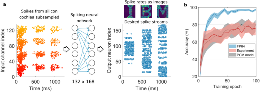
The image presents a diagram illustrating a spiking neural network setup alongside a chart showing the training accuracy of different models over training epochs. The diagram depicts the flow of spikes from a silicon cochlea through a spiking neural network to desired spike streams. The chart shows the accuracy (%) of three models (FP64, Experiment, and PCM model) as a function of training epoch.
### Components/Axes
**Diagram (a):**
* **Left Plot:** Scatter plot of "Spikes from silicon cochlea subsampled". X-axis: "Time (ms)", ranging from 0 to 1000. Y-axis: "Input channel index", ranging from 0 to 120. Data points are colored orange and red.
* **Center Diagram:** Representation of a "Spiking neural network". It shows a network with 132 input nodes and 168 output nodes, connected by lines representing synaptic connections.
* **Right Plot:** Scatter plot of "Desired spike streams". X-axis: "Time (ms)", ranging from 0 to 1000. Y-axis: "Output neuron index", ranging from 0 to 150. Data points are colored blue.
* **Top-Right:** Four images representing "Spike rates as images", each a 4x4 grid of colored squares.
**Chart (b):**
* X-axis: "Training epoch", ranging from 0 to 100.
* Y-axis: "Accuracy (%)", ranging from 20 to 100.
* Three lines representing different models:
* FP64 (teal)
* Experiment (red)
* PCM model (grey)
* Shaded areas around each line represent the standard deviation or confidence interval.
### Detailed Analysis or Content Details
**Diagram (a):**
* The left plot shows two distinct clusters of orange and red points, suggesting two different spike patterns over time. The orange points are concentrated between 0-500ms and 80-120 input channel index, while the red points are concentrated between 500-1000ms and 0-40 input channel index.
* The spiking neural network diagram shows a fully connected layer with 132 input nodes and 168 output nodes.
* The right plot shows a dense pattern of blue points, indicating a consistent stream of spikes across all output neurons and time.
**Chart (b):**
* **FP64:** The teal line starts at approximately 50% accuracy at epoch 0 and rises sharply to around 95% accuracy by epoch 50. It plateaus around 95-98% for the remainder of the training epochs.
* **Experiment:** The red line starts at approximately 45% accuracy at epoch 0 and rises steadily to around 85% accuracy by epoch 100. The shaded area around the line indicates a significant amount of variability in the accuracy.
* **PCM model:** The grey line starts at approximately 40% accuracy at epoch 0 and rises steadily to around 75% accuracy by epoch 100. The shaded area around the line indicates a significant amount of variability in the accuracy.
### Key Observations
* The FP64 model achieves the highest accuracy and converges quickly.
* The Experiment and PCM models show slower convergence and lower overall accuracy.
* The Experiment and PCM models have larger variability in accuracy compared to the FP64 model.
* The spike patterns in the silicon cochlea (left plot) are distinct, suggesting different auditory stimuli.
### Interpretation
The diagram illustrates a computational model of auditory processing, where spikes from a silicon cochlea are processed by a spiking neural network to generate desired spike streams. The chart shows the training accuracy of different models used to implement this network. The FP64 model, likely a high-precision floating-point model, demonstrates superior performance, suggesting that higher precision is beneficial for training this type of network. The Experiment and PCM models, potentially lower-precision or alternative implementations, show lower accuracy and greater variability, indicating challenges in achieving comparable performance with these approaches. The difference in accuracy between the models could be due to the limitations of lower-precision arithmetic or the specific architecture of the PCM model. The distinct spike patterns in the silicon cochlea suggest that the network is capable of processing different auditory stimuli. The overall results suggest that while spiking neural networks hold promise for auditory processing, careful consideration must be given to the precision and architecture of the models used to implement them.