## Diagram: Spiking Neural Network Processing and Training Performance
### Overview
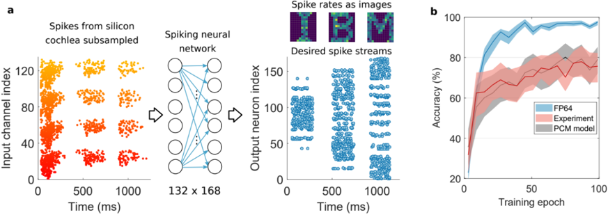
The image contains two primary components:
1. **Part a**: A spiking neural network (SNN) architecture processing subsampled cochlear spikes into desired spike streams.
2. **Part b**: A line graph comparing training accuracy across epochs for three models (FP64, Experiment, PCM).
---
### Components/Axes
#### Part a
- **Left Panel**:
- **Y-axis**: Input channel index (0–120).
- **X-axis**: Time (ms, 0–1000).
- **Data**: Heatmap of spike activity (red = low rate, yellow = high rate) from a silicon cochlea subsampled.
- **Center Diagram**:
- **Neural Network**: 132×168 connections (input to output layer).
- **Arrows**: Indicate flow from input spikes to output neuron indices.
- **Right Panel**:
- **Y-axis**: Output neuron index (0–150).
- **X-axis**: Time (ms, 0–1000).
- **Data**: Desired spike streams (blue dots) and spike rates visualized as images (labeled "IBM" three times).
#### Part b
- **X-axis**: Training epoch (0–100).
- **Y-axis**: Accuracy (%) (20–100).
- **Legend**:
- **Blue**: FP64 (solid line).
- **Red**: Experiment (dashed line with shaded confidence interval).
- **Gray**: PCM model (dotted line with shaded confidence interval).
---
### Detailed Analysis
#### Part a
- **Spike Distribution**:
- Spikes cluster in specific input channels (e.g., channels 0–20 show high activity in early time bins).
- Subsampling reduces temporal resolution (e.g., sparse spikes in later time bins).
- **Neural Network**:
- 132 input neurons → 168 output neurons.
- Output neuron indices range from 0 to 150, with sparse activation patterns.
- **Desired Spike Streams**:
- Blue dots represent target spike timings.
- IBM images (likely placeholders) suggest categorical spike patterns.
#### Part b
- **FP64 Model**:
- Starts at ~20% accuracy (epoch 0), rises sharply to ~95% by epoch 50, then plateaus.
- Confidence interval narrows as training progresses.
- **Experiment Model**:
- Begins at ~30%, fluctuates between 50–80%, with wider confidence intervals.
- Peaks at ~85% by epoch 100.
- **PCM Model**:
- Starts at ~20%, rises slowly to ~60%, with the widest confidence intervals.
---
### Key Observations
1. **Part a**:
- The SNN maps cochlear spike patterns (input) to structured output streams, suggesting temporal coding.
- IBM images may represent predefined spike templates for specific tasks.
2. **Part b**:
- FP64 outperforms both Experiment and PCM models, indicating higher precision.
- PCM model’s lower accuracy and wider confidence intervals suggest instability or approximation errors.
---
### Interpretation
- **Neural Network Functionality**:
The SNN transforms raw cochlear spike data into discrete output streams, likely for tasks like speech recognition or auditory processing. The IBM images may encode specific phonetic or rhythmic patterns.
- **Training Performance**:
- FP64’s dominance highlights the importance of numerical precision in training SNNs.
- The Experiment model bridges FP64 and PCM, suggesting real-world implementations face trade-offs between accuracy and computational constraints.
- PCM’s poor performance implies it may lack the capacity or optimization to handle complex spike dynamics.
- **Critical Insights**:
- Subsampling cochlear data risks losing temporal resolution, which the SNN partially compensates for via learned spike timing.
- The PCM model’s wide confidence intervals indicate high variance in training, possibly due to hardware limitations or simplified architecture.
- FP64’s plateau at ~95% suggests near-optimal performance for this task, leaving little room for improvement.
- **Anomalies**:
- The IBM images in part a are ambiguous; their repetition may indicate a placeholder or error in the diagram.
- The Experiment model’s fluctuating accuracy could reflect dataset variability or overfitting.