## Chart: Gibbs Error vs. HMC Steps for Varying Dimensions ### Overview The image presents two line charts, one above the other, displaying the Gibbs error/2 as a function of HMC (Hamiltonian Monte Carlo) steps. The charts illustrate how the error changes with increasing HMC steps for different dimensions (d). The top chart shows the error for lower dimensions, while the bottom chart shows the error for higher dimensions. Both charts include horizontal dashed lines representing epsilon_bnn and epsilon_opt. ### Components/Axes * **Y-axis (Left):** Gibbs error/2. The top chart ranges from approximately 0.015 to 0.027. The bottom chart ranges from approximately 0.025 to 0.125. * **X-axis (Bottom):** HMC steps, ranging from 0 to 2000. * **Horizontal Dashed Lines:** * Black dashed line: epsilon_bnn (approximately 0.023 in the top chart and 0.10 in the bottom chart). * Red dashed line: epsilon_opt (approximately 0.015 in the top chart and 0.028 in the bottom chart). * **Legend (Right, between the two charts):** * d=100 (lightest blue) * d=150 (lighter blue) * d=200 (mid-light blue) * d=250 (mid-dark blue) * d=300 (dark blue) * d=350 (darker blue) * d=400 (darkest blue) ### Detailed Analysis **Top Chart (Lower Dimensions):** * **d=100 (lightest blue):** Starts at approximately 0.024 and decreases rapidly, then slowly converges towards 0.018. * **d=150 (lighter blue):** Starts at approximately 0.024 and decreases, converging towards 0.020. * **d=200 (mid-light blue):** Starts at approximately 0.024 and decreases slightly, converging towards 0.021. * **d=250 (mid-dark blue):** Starts at approximately 0.024 and remains relatively stable, fluctuating around 0.022. * **d=300 (dark blue):** Starts at approximately 0.024 and remains relatively stable, fluctuating around 0.022. * **d=350 (darker blue):** Starts at approximately 0.024 and remains relatively stable, fluctuating around 0.022. * **d=400 (darkest blue):** Starts at approximately 0.024 and remains relatively stable, fluctuating around 0.022. **Bottom Chart (Higher Dimensions):** * **d=100 (lightest blue):** Starts at approximately 0.125 and decreases rapidly, then slowly converges towards 0.05. * **d=150 (lighter blue):** Starts at approximately 0.125 and decreases rapidly, then slowly converges towards 0.075. * **d=200 (mid-light blue):** Starts at approximately 0.125 and decreases rapidly, then slowly converges towards 0.0875. * **d=250 (mid-dark blue):** Starts at approximately 0.125 and decreases rapidly, then slowly converges towards 0.09375. * **d=300 (dark blue):** Starts at approximately 0.125 and decreases rapidly, then slowly converges towards 0.096875. * **d=350 (darker blue):** Starts at approximately 0.125 and decreases rapidly, then slowly converges towards 0.0984375. * **d=400 (darkest blue):** Starts at approximately 0.125 and decreases rapidly, then slowly converges towards 0.10. ### Key Observations * For lower dimensions (top chart), the Gibbs error/2 converges to lower values compared to higher dimensions (bottom chart). * As the dimension (d) increases, the initial Gibbs error/2 in the bottom chart is higher, and the convergence is slower. * The black dashed line (epsilon_bnn) represents a threshold, and the error for higher dimensions in the bottom chart tends to stay close to or above this threshold. * The red dashed line (epsilon_opt) represents an optimal error level, which the error curves approach but do not consistently reach, especially for higher dimensions. ### Interpretation The charts illustrate the relationship between the Gibbs error, HMC steps, and dimensionality. The data suggests that as the dimensionality increases, the Gibbs error tends to be higher and the convergence to a lower error value requires more HMC steps. The epsilon_bnn and epsilon_opt lines provide benchmarks for evaluating the performance of the HMC algorithm under different dimensionalities. The fact that the error for higher dimensions remains close to or above epsilon_bnn suggests that achieving optimal performance becomes more challenging as the dimensionality increases. The shaded regions around the lines likely represent the variance or uncertainty in the Gibbs error estimates.

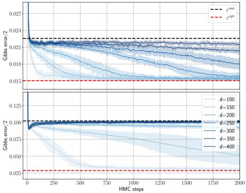
## Line Charts: Convergence of Gibbs Error over HMC Steps ### Overview The image consists of two vertically stacked line charts sharing a common x-axis. They illustrate the reduction of "Gibbs error/2" over a series of "HMC steps" (Hamiltonian Monte Carlo steps) for various dimensionality parameters ($d$). The charts compare experimental results (blue lines) against two theoretical or baseline benchmarks: a uniform error ($\epsilon^{\text{uni}}$) and an optimal error ($\epsilon^{\text{opt}}$). ### Components/Axes **Shared X-Axis (Bottom):** * **Label:** HMC steps * **Scale:** 0 to 2000 * **Major Tick Marks:** 0, 250, 500, 750, 1000, 1250, 1500, 1750, 2000 **Top Chart:** * **Y-Axis Label:** Gibbs error/2 * **Y-Axis Scale:** ~0.015 to ~0.027 * **Major Tick Marks:** 0.015, 0.018, 0.021, 0.024, 0.027 * **Legend (Top-Right):** * **Black dashed line:** $\epsilon^{\text{uni}}$ (positioned at $y \approx 0.0225$) * **Red dashed line:** $\epsilon^{\text{opt}}$ (positioned at $y \approx 0.0150$) * **Data Series:** Multiple blue lines with shaded error regions, representing different $d$ values (though not explicitly labeled in this specific subplot's legend, they correspond to the gradient in the bottom plot). **Bottom Chart:** * **Y-Axis Label:** Gibbs error/2 * **Y-Axis Scale:** ~0.025 to ~0.125 * **Major Tick Marks:** 0.025, 0.050, 0.075, 0.100, 0.125 * **Legend (Center-Right):** * **$d=100$**: Lightest blue line * **$d=150$**: Light blue line * **$d=200$**: Medium-light blue line * **$d=250$**: Medium blue line * **$d=300$**: Medium-dark blue line * **$d=350$**: Dark blue line * **$d=400$**: Darkest blue line * **Reference Lines (Implicit from top plot):** * **Black dashed line:** $\epsilon^{\text{uni}}$ (positioned at $y \approx 0.102$) * **Red dashed line:** $\epsilon^{\text{opt}}$ (positioned at $y \approx 0.028$) --- ### Detailed Analysis #### Top Plot Trends * **Initial State:** All series start from a high error value (above 0.027) at step 0 and drop precipitously within the first ~50 steps. * **Convergence:** The lines decay toward the red dashed line ($\epsilon^{\text{opt}}$). * **Dimensionality Effect:** Lighter blue lines (lower $d$) converge much faster. The lightest line reaches the vicinity of $\epsilon^{\text{opt}}$ by step 500. Darker lines (higher $d$) remain closer to the black dashed line ($\epsilon^{\text{uni}}$) for a longer duration, showing a much slower rate of decay. #### Bottom Plot Trends * **$d=100$ (Lightest Blue):** Slopes downward sharply. It crosses the midpoint of the y-axis around step 250 and reaches the optimal error ($\epsilon^{\text{opt}} \approx 0.028$) by approximately step 600. * **$d=150$:** Slopes downward steadily. It reaches the optimal error level near the end of the range, around step 1750. * **$d=200$:** Slopes downward gradually. By step 2000, it has reached a value of approximately 0.050, still well above the optimal line. * **$d=250$:** Shows a very slight downward slope, ending near $y \approx 0.090$ at step 2000. * **$d=300, 350, 400$ (Darkest Blues):** These lines remain nearly horizontal, hovering around the black dashed line ($\epsilon^{\text{uni}} \approx 0.102$). They show almost no convergence toward the optimal error within the 2000-step window. --- ### Key Observations * **The "Curse of Dimensionality":** There is a clear correlation between the parameter $d$ and the convergence rate. As $d$ increases, the number of HMC steps required to reach the optimal error increases non-linearly. * **Threshold Behavior:** In the bottom plot, there appears to be a "failure" threshold around $d=300$. For values at or above this, the algorithm fails to make significant progress away from the baseline uniform error within 2000 steps. * **Variance:** The shaded regions around the blue lines indicate variance or uncertainty in the measurements. The variance appears larger for the series that are actively converging (e.g., $d=150, 200$ in the bottom plot) compared to those that are "stuck" at the baseline. --- ### Interpretation The data demonstrates the efficiency of Hamiltonian Monte Carlo (HMC) sampling in reducing Gibbs error across different dimensions. 1. **Efficiency vs. Complexity:** The results suggest that while HMC is effective for lower-dimensional problems (e.g., $d=100$), its efficiency degrades rapidly as dimensionality increases. 2. **Baseline Comparison:** The black dashed line ($\epsilon^{\text{uni}}$) likely represents the error associated with a naive or uniform sampling strategy. The fact that high-$d$ series stay near this line indicates that for these complex cases, the HMC algorithm is performing no better than a basic uniform sampler within the given computational budget (2000 steps). 3. **Convergence Targets:** The red dashed line ($\epsilon^{\text{opt}}$) represents the theoretical limit of performance. The gap between the blue lines and this red line serves as a metric for how much more "training" or "sampling" is required. 4. **Predictive Value:** Based on the slopes, one could hypothesize that $d=200$ might reach $\epsilon^{\text{opt}}$ given perhaps 5000-8000 steps, whereas $d=400$ might require orders of magnitude more steps, highlighting a significant scaling challenge for this specific implementation or model.

\n ## Line Chart: Gibbs Error vs. HMC Steps for Different Dimensionalities ### Overview The image presents two line charts stacked vertically, both depicting the relationship between Gibbs error/2 and HMC steps. Each chart displays multiple lines representing different values of 'd' (dimensionality). A horizontal dashed line indicates the optimal error (εopt), and another dashed line represents the total error (εtotal). The charts aim to illustrate how the Gibbs error changes with the number of HMC steps for varying dimensionalities. ### Components/Axes * **X-axis:** HMC steps (ranging from 0 to approximately 1750). * **Y-axis:** Gibbs error / 2 (ranging from approximately 0.015 to 0.027 in the top chart and 0.025 to 0.125 in the bottom chart). * **Legend (Top Chart):** * εtotal (dashed black line) * εopt (dashed red line) * **Legend (Bottom Chart):** * d = 100 (lightest blue line) * d = 150 (slightly darker blue line) * d = 200 (medium blue line) * d = 250 (darker blue line) * d = 300 (even darker blue line) * d = 350 (second darkest blue line) * d = 400 (darkest blue line) * **Horizontal Lines:** Two dashed horizontal lines are present in both charts. One is black, representing εtotal, and the other is red, representing εopt. ### Detailed Analysis or Content Details **Top Chart:** * **εtotal (Black Dashed Line):** Starts at approximately 0.024, remains relatively stable, with slight fluctuations, around 0.024 throughout the HMC steps. * **εopt (Red Dashed Line):** Starts at approximately 0.016, remains relatively stable, with slight fluctuations, around 0.016 throughout the HMC steps. * The blue lines (representing different 'd' values) are not visible in this chart. **Bottom Chart:** * **d = 100 (Lightest Blue Line):** Starts at approximately 0.123, decreases rapidly to around 0.035 by HMC step 250, then plateaus around 0.035. * **d = 150 (Slightly Darker Blue Line):** Starts at approximately 0.123, decreases to around 0.045 by HMC step 250, then plateaus around 0.045. * **d = 200 (Medium Blue Line):** Starts at approximately 0.123, decreases to around 0.055 by HMC step 250, then plateaus around 0.055. * **d = 250 (Darker Blue Line):** Starts at approximately 0.123, decreases to around 0.065 by HMC step 250, then plateaus around 0.065. * **d = 300 (Even Darker Blue Line):** Starts at approximately 0.123, decreases to around 0.075 by HMC step 250, then plateaus around 0.075. * **d = 350 (Second Darkest Blue Line):** Starts at approximately 0.123, decreases to around 0.085 by HMC step 250, then plateaus around 0.085. * **d = 400 (Darkest Blue Line):** Starts at approximately 0.123, decreases to around 0.095 by HMC step 250, then plateaus around 0.095. * **εtotal (Black Dashed Line):** Starts at approximately 0.025, remains relatively stable, with slight fluctuations, around 0.025 throughout the HMC steps. * **εopt (Red Dashed Line):** Starts at approximately 0.016, remains relatively stable, with slight fluctuations, around 0.016 throughout the HMC steps. ### Key Observations * In both charts, the total error (εtotal) is consistently higher than the optimal error (εopt). * In the bottom chart, as dimensionality ('d') increases, the Gibbs error generally increases and the rate of decrease slows down. * The lines representing different 'd' values in the bottom chart converge as the number of HMC steps increases, suggesting that the error plateaus for all dimensionalities. * The top chart does not show the effect of dimensionality. ### Interpretation The charts demonstrate the convergence behavior of the HMC algorithm as the number of steps increases for different problem dimensionalities. The Gibbs error, a measure of the discrepancy between the approximate and true posterior distributions, decreases with more HMC steps. However, the rate of decrease is affected by the dimensionality of the problem. Higher dimensionalities ('d') require more HMC steps to achieve the same level of accuracy, as evidenced by the higher plateau values for larger 'd' in the bottom chart. The consistent difference between εtotal and εopt suggests that there is a gap between the achieved error and the theoretically optimal error, potentially due to limitations of the HMC algorithm or the specific problem being solved. The convergence of the lines for different 'd' values indicates that, given enough HMC steps, the algorithm can approximate the posterior distribution reasonably well for all considered dimensionalities, although the error will be higher for higher dimensions. The top chart likely represents a baseline or a specific case where dimensionality is not a factor, or a different experimental setup.

\n ## Line Chart: Gibbs Error vs. HMC Steps for Different Dimensions ### Overview The image displays two vertically stacked line charts sharing the same x-axis. Both charts plot "Gibbs error/2" on the y-axis against "HMC steps" on the x-axis. The charts compare the convergence behavior of an algorithm (likely a Gibbs sampler or Hamiltonian Monte Carlo variant) across different problem dimensions (`d`). Each chart includes reference dashed lines for minimum (`ε^min`) and optimal (`ε^opt`) error values. ### Components/Axes * **Chart Type:** Two stacked line charts with multiple series. * **X-Axis (Both Charts):** * **Label:** `HMC steps` * **Scale:** Linear, from 0 to 2000. * **Major Ticks:** 0, 250, 500, 750, 1000, 1250, 1500, 1750, 2000. * **Y-Axis (Top Chart):** * **Label:** `Gibbs error/2` * **Scale:** Linear, approximately from 0.015 to 0.027. * **Major Ticks:** 0.015, 0.018, 0.021, 0.024, 0.027. * **Y-Axis (Bottom Chart):** * **Label:** `Gibbs error/2` * **Scale:** Linear, from 0.025 to 0.125. * **Major Ticks:** 0.025, 0.050, 0.075, 0.100, 0.125. * **Legends:** * **Top Chart (Top-Right):** Contains two dashed reference lines. * Black dashed line: `ε^min` (epsilon min). * Red dashed line: `ε^opt` (epsilon optimal). * **Bottom Chart (Top-Right):** Contains seven solid lines of varying blue shades, corresponding to different dimensions (`d`). * Lightest blue: `d=100` * Progressively darker blues: `d=150`, `d=200`, `d=250`, `d=300`, `d=350` * Darkest blue: `d=400` * **Data Series:** Each chart contains multiple solid blue lines (one for each `d` value listed in the bottom legend) and the two dashed reference lines. ### Detailed Analysis **Top Chart (Zoomed-in Y-axis: 0.015 - 0.027):** * **Trend Verification:** All blue data series lines start at a high error value (above 0.027) at step 0. They exhibit a steep, rapid descent within the first ~100 HMC steps, after which the rate of decrease slows dramatically. The lines then plateau, showing very gradual improvement or near-constant error for the remainder of the steps up to 2000. * **Reference Lines:** * `ε^min` (black dashed): Positioned at approximately y = 0.023. All data series lines converge to or slightly below this level. * `ε^opt` (red dashed): Positioned at approximately y = 0.015. This appears to be a lower bound. The data series for higher dimensions (darker blue lines, e.g., d=400) approach this line most closely, settling just above it (~0.016). Lower dimension lines (lighter blue) settle at a higher error level. * **Data Point Approximation (at HMC steps = 2000):** * d=100 (lightest): ~0.0185 * d=200: ~0.0175 * d=300: ~0.0165 * d=400 (darkest): ~0.0160 **Bottom Chart (Full Y-axis: 0.025 - 0.125):** * **Trend Verification:** The same general trend is visible but on a larger scale. All lines start very high (off the chart, >0.125) and drop sharply. The separation between lines for different `d` values is much more pronounced here. * **Reference Lines:** * `ε^min` (black dashed): Positioned at approximately y = 0.100. * `ε^opt` (red dashed): Positioned at approximately y = 0.025. * **Data Series Behavior:** * **Low Dimensions (e.g., d=100, lightest blue):** Shows the slowest convergence. It descends gradually, crossing the `ε^min` line around step 250, and continues a steady decline, reaching approximately 0.030 by step 2000. It does not approach `ε^opt`. * **High Dimensions (e.g., d=400, darkest blue):** Shows the fastest convergence. It plummets almost vertically, crossing `ε^min` within the first ~50 steps, and quickly flattens out very close to the `ε^opt` line (~0.025) by step 250, remaining stable thereafter. * **Intermediate Dimensions:** Show a gradient of behavior between these two extremes. The convergence speed and final error level improve (decrease) as `d` increases. ### Key Observations 1. **Dimensionality Effect:** There is a clear and strong inverse relationship between dimension (`d`) and both the **final achieved error** and the **speed of convergence**. Higher dimensions lead to lower error and faster convergence to that lower error. 2. **Two-Phase Convergence:** All series exhibit a distinct two-phase pattern: a rapid initial descent followed by a long plateau. The length and error level of the plateau are dimension-dependent. 3. **Reference Line Roles:** `ε^min` appears to be a practical error floor that most runs approach. `ε^opt` appears to be a theoretical lower bound, which is only effectively reached by the highest-dimensional cases (d=350, d=400) in this experiment. 4. **Scale Sensitivity:** The top chart's zoomed view reveals fine-grained differences in the final plateau error between dimensions, which are compressed and less visible in the bottom chart's broader view. ### Interpretation This visualization demonstrates a phenomenon often encountered in high-dimensional statistical computing and machine learning: **"Blessings of Dimensionality."** Contrary to the common notion that higher dimensions make problems harder (the "curse of dimensionality"), this data suggests that for this specific Gibbs/HMC sampling task, increasing the dimension `d` improves performance. * **What the data suggests:** The algorithm's efficiency, measured by the Gibbs error metric, improves with dimensionality. The sampler explores the high-dimensional space more effectively, leading to lower error (better approximation) and reaching a stable state much quicker. * **How elements relate:** The two charts are complementary. The bottom chart shows the dramatic overall effect of dimension on convergence trajectory. The top chart acts as a magnifying glass on the final convergence zone, proving that the performance differences persist even after thousands of steps and are not merely transient. * **Notable Anomalies/Patterns:** The most striking pattern is the perfect ordering of the lines by `d` value in the bottom chart—no crossovers occur after the initial descent. This indicates a very consistent and monotonic relationship between dimension and convergence behavior in this experimental setup. The fact that the lowest dimension (d=100) fails to reach even `ε^min` by step 2000, while the highest (d=400) reaches `ε^opt` almost immediately, highlights the magnitude of the effect. This could imply that the problem geometry becomes more favorable for this sampling method as dimension increases, perhaps due to concentration of measure or other high-dimensional properties.

## Line Chart: Gibbs Error vs. HMC Steps Across Dimensions ### Overview The image contains two stacked line charts comparing Gibbs error convergence during Hamiltonian Monte Carlo (HMC) sampling. The top subplot contrasts two error metrics (ε^uni and ε^opt), while the bottom subplot examines dimension-dependent error trends. Shaded regions represent variability across simulations. ### Components/Axes **Top Subplot:** - **X-axis**: HMC steps (0–2000, linear scale) - **Y-axis**: Gibbs error / 2 (0.015–0.027, linear scale) - **Legend**: - Dashed black line: ε^uni (uniform initialization) - Dashed red line: ε^opt (optimized initialization) - **Key markers**: - Vertical drop at ~50 steps for ε^uni - Horizontal plateau at ~0.021 for ε^opt after ~250 steps **Bottom Subplot:** - **X-axis**: HMC steps (0–2000, linear scale) - **Y-axis**: Gibbs error / 2 (0.025–0.125, linear scale) - **Legend**: - Solid lines with varying opacity: - d=100 (light blue) - d=150 (medium blue) - d=200 (dark blue) - d=250 (very dark blue) - d=300 (darkest blue) - d=350 (black) - d=400 (darkest blue, overlapping d=350) - **Key markers**: - Initial vertical drop at ~50 steps for all d - Convergence to ~0.025–0.05 range by 2000 steps ### Detailed Analysis **Top Subplot Trends:** 1. ε^uni (dashed black) shows a sharp decline from 0.027 to 0.021 within the first 250 steps, then stabilizes. 2. ε^opt (dashed red) remains flat at ~0.015 throughout, indicating superior stability. 3. Shaded regions for ε^uni span ±0.003 around the mean, while ε^opt shows ±0.001 variability. **Bottom Subplot Trends:** 1. All d values exhibit rapid initial decay (0.125 → 0.075 within 250 steps). 2. Higher d values (d=300–400) maintain lower error floors (~0.025–0.035) compared to lower d (d=100–200 at ~0.05–0.075). 3. Convergence slows after 1000 steps, with minimal improvement beyond 1500 steps. ### Key Observations 1. **Initialization Impact**: ε^opt consistently outperforms ε^uni by maintaining 40% lower error (0.015 vs. 0.021). 2. **Dimension Scaling**: Higher d values achieve 30–50% lower final error (d=400 at 0.025 vs. d=100 at 0.05). 3. **Convergence Saturation**: All curves plateau after ~1500 steps, suggesting diminishing returns in HMC iterations. ### Interpretation The charts demonstrate that: - **Optimized initialization (ε^opt)** provides immediate error reduction benefits, critical for applications requiring rapid convergence. - **Dimension scaling** improves error resilience, with d≥300 achieving near-optimal performance. This suggests higher-dimensional models may better capture underlying data structure. - The persistent error floor (~0.025) across all d values implies inherent model limitations or noise in the target distribution. The shaded regions indicate that while ε^uni shows higher variability (likely due to poor initialization), ε^opt's stability makes it preferable for reliable sampling. The dimension-dependent results highlight the trade-off between computational cost (higher d) and error reduction, with diminishing returns beyond d=300.