\n
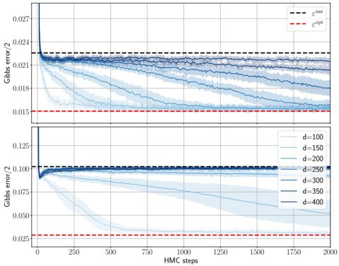
## Line Chart: Gibbs Error vs. HMC Steps for Different Dimensionalities
### Overview
The image presents two line charts stacked vertically, both depicting the relationship between Gibbs error/2 and HMC steps. Each chart displays multiple lines representing different values of 'd' (dimensionality). A horizontal dashed line indicates the optimal error (εopt), and another dashed line represents the total error (εtotal). The charts aim to illustrate how the Gibbs error changes with the number of HMC steps for varying dimensionalities.
### Components/Axes
* **X-axis:** HMC steps (ranging from 0 to approximately 1750).
* **Y-axis:** Gibbs error / 2 (ranging from approximately 0.015 to 0.027 in the top chart and 0.025 to 0.125 in the bottom chart).
* **Legend (Top Chart):**
* εtotal (dashed black line)
* εopt (dashed red line)
* **Legend (Bottom Chart):**
* d = 100 (lightest blue line)
* d = 150 (slightly darker blue line)
* d = 200 (medium blue line)
* d = 250 (darker blue line)
* d = 300 (even darker blue line)
* d = 350 (second darkest blue line)
* d = 400 (darkest blue line)
* **Horizontal Lines:** Two dashed horizontal lines are present in both charts. One is black, representing εtotal, and the other is red, representing εopt.
### Detailed Analysis or Content Details
**Top Chart:**
* **εtotal (Black Dashed Line):** Starts at approximately 0.024, remains relatively stable, with slight fluctuations, around 0.024 throughout the HMC steps.
* **εopt (Red Dashed Line):** Starts at approximately 0.016, remains relatively stable, with slight fluctuations, around 0.016 throughout the HMC steps.
* The blue lines (representing different 'd' values) are not visible in this chart.
**Bottom Chart:**
* **d = 100 (Lightest Blue Line):** Starts at approximately 0.123, decreases rapidly to around 0.035 by HMC step 250, then plateaus around 0.035.
* **d = 150 (Slightly Darker Blue Line):** Starts at approximately 0.123, decreases to around 0.045 by HMC step 250, then plateaus around 0.045.
* **d = 200 (Medium Blue Line):** Starts at approximately 0.123, decreases to around 0.055 by HMC step 250, then plateaus around 0.055.
* **d = 250 (Darker Blue Line):** Starts at approximately 0.123, decreases to around 0.065 by HMC step 250, then plateaus around 0.065.
* **d = 300 (Even Darker Blue Line):** Starts at approximately 0.123, decreases to around 0.075 by HMC step 250, then plateaus around 0.075.
* **d = 350 (Second Darkest Blue Line):** Starts at approximately 0.123, decreases to around 0.085 by HMC step 250, then plateaus around 0.085.
* **d = 400 (Darkest Blue Line):** Starts at approximately 0.123, decreases to around 0.095 by HMC step 250, then plateaus around 0.095.
* **εtotal (Black Dashed Line):** Starts at approximately 0.025, remains relatively stable, with slight fluctuations, around 0.025 throughout the HMC steps.
* **εopt (Red Dashed Line):** Starts at approximately 0.016, remains relatively stable, with slight fluctuations, around 0.016 throughout the HMC steps.
### Key Observations
* In both charts, the total error (εtotal) is consistently higher than the optimal error (εopt).
* In the bottom chart, as dimensionality ('d') increases, the Gibbs error generally increases and the rate of decrease slows down.
* The lines representing different 'd' values in the bottom chart converge as the number of HMC steps increases, suggesting that the error plateaus for all dimensionalities.
* The top chart does not show the effect of dimensionality.
### Interpretation
The charts demonstrate the convergence behavior of the HMC algorithm as the number of steps increases for different problem dimensionalities. The Gibbs error, a measure of the discrepancy between the approximate and true posterior distributions, decreases with more HMC steps. However, the rate of decrease is affected by the dimensionality of the problem. Higher dimensionalities ('d') require more HMC steps to achieve the same level of accuracy, as evidenced by the higher plateau values for larger 'd' in the bottom chart.
The consistent difference between εtotal and εopt suggests that there is a gap between the achieved error and the theoretically optimal error, potentially due to limitations of the HMC algorithm or the specific problem being solved. The convergence of the lines for different 'd' values indicates that, given enough HMC steps, the algorithm can approximate the posterior distribution reasonably well for all considered dimensionalities, although the error will be higher for higher dimensions. The top chart likely represents a baseline or a specific case where dimensionality is not a factor, or a different experimental setup.