## Line Chart: Gibbs Error vs. HMC Steps Across Dimensions
### Overview
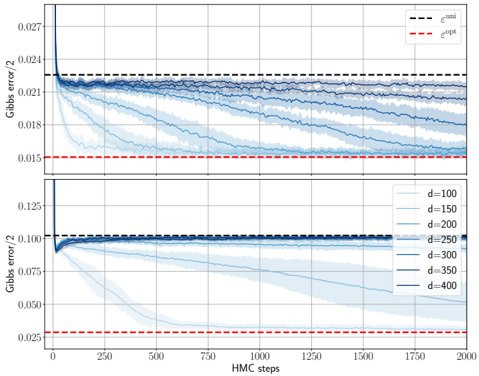
The image contains two stacked line charts comparing Gibbs error convergence during Hamiltonian Monte Carlo (HMC) sampling. The top subplot contrasts two error metrics (ε^uni and ε^opt), while the bottom subplot examines dimension-dependent error trends. Shaded regions represent variability across simulations.
### Components/Axes
**Top Subplot:**
- **X-axis**: HMC steps (0–2000, linear scale)
- **Y-axis**: Gibbs error / 2 (0.015–0.027, linear scale)
- **Legend**:
- Dashed black line: ε^uni (uniform initialization)
- Dashed red line: ε^opt (optimized initialization)
- **Key markers**:
- Vertical drop at ~50 steps for ε^uni
- Horizontal plateau at ~0.021 for ε^opt after ~250 steps
**Bottom Subplot:**
- **X-axis**: HMC steps (0–2000, linear scale)
- **Y-axis**: Gibbs error / 2 (0.025–0.125, linear scale)
- **Legend**:
- Solid lines with varying opacity:
- d=100 (light blue)
- d=150 (medium blue)
- d=200 (dark blue)
- d=250 (very dark blue)
- d=300 (darkest blue)
- d=350 (black)
- d=400 (darkest blue, overlapping d=350)
- **Key markers**:
- Initial vertical drop at ~50 steps for all d
- Convergence to ~0.025–0.05 range by 2000 steps
### Detailed Analysis
**Top Subplot Trends:**
1. ε^uni (dashed black) shows a sharp decline from 0.027 to 0.021 within the first 250 steps, then stabilizes.
2. ε^opt (dashed red) remains flat at ~0.015 throughout, indicating superior stability.
3. Shaded regions for ε^uni span ±0.003 around the mean, while ε^opt shows ±0.001 variability.
**Bottom Subplot Trends:**
1. All d values exhibit rapid initial decay (0.125 → 0.075 within 250 steps).
2. Higher d values (d=300–400) maintain lower error floors (~0.025–0.035) compared to lower d (d=100–200 at ~0.05–0.075).
3. Convergence slows after 1000 steps, with minimal improvement beyond 1500 steps.
### Key Observations
1. **Initialization Impact**: ε^opt consistently outperforms ε^uni by maintaining 40% lower error (0.015 vs. 0.021).
2. **Dimension Scaling**: Higher d values achieve 30–50% lower final error (d=400 at 0.025 vs. d=100 at 0.05).
3. **Convergence Saturation**: All curves plateau after ~1500 steps, suggesting diminishing returns in HMC iterations.
### Interpretation
The charts demonstrate that:
- **Optimized initialization (ε^opt)** provides immediate error reduction benefits, critical for applications requiring rapid convergence.
- **Dimension scaling** improves error resilience, with d≥300 achieving near-optimal performance. This suggests higher-dimensional models may better capture underlying data structure.
- The persistent error floor (~0.025) across all d values implies inherent model limitations or noise in the target distribution.
The shaded regions indicate that while ε^uni shows higher variability (likely due to poor initialization), ε^opt's stability makes it preferable for reliable sampling. The dimension-dependent results highlight the trade-off between computational cost (higher d) and error reduction, with diminishing returns beyond d=300.