TECHNICAL ASSET FINGERPRINT
16c4a36b9a5c2d9fe0b8159c
Click to view fullscreen
Press ESC or click to close
FOUND IN PAPERS
EXPERT: healer-alpha-free VERSION 1
RUNTIME: free/openrouter/healer-alpha
INTEL_VERIFIED
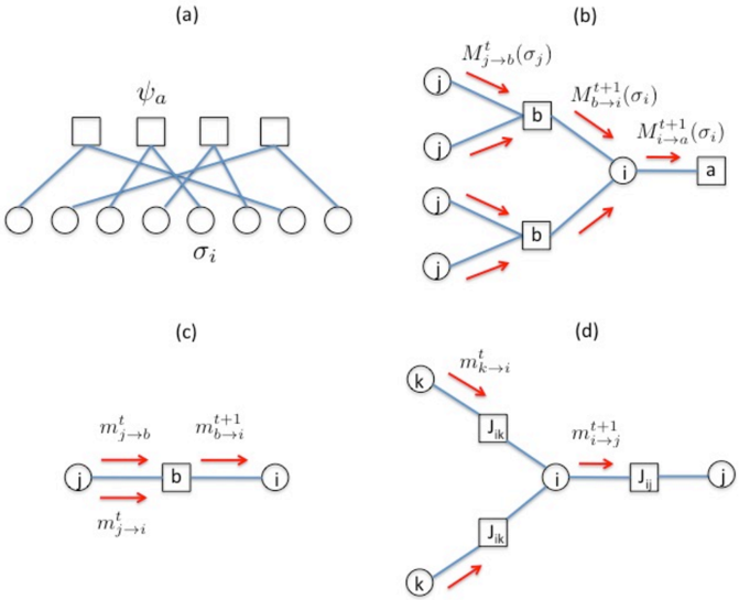
## Diagram Set: Graphical Model and Message-Passing Notation
### Overview
The image contains four distinct but related technical diagrams, labeled (a) through (d). These diagrams illustrate concepts from probabilistic graphical models, specifically factor graphs and message-passing algorithms (like belief propagation). The diagrams use a consistent visual language: circular nodes represent variables, square nodes represent factors or functions, blue lines represent edges in the graph, and red arrows represent the flow of messages between nodes.
### Components/Axes
The image is a composite of four sub-figures. There are no traditional chart axes. The key components are:
* **Node Types:**
* **Circular Nodes:** Represent variables. Labeled with indices like `i`, `j`, `k`.
* **Square Nodes:** Represent factors or functions. Labeled with identifiers like `a`, `b`, `J_ik`, `J_ij`, or function symbols like `ψ_a`.
* **Edge Types:**
* **Blue Lines:** Undirected edges connecting variable and factor nodes, defining the graph structure.
* **Red Arrows:** Directed edges representing the flow of messages. Each has an associated label.
* **Message Labels:** Mathematical notation indicating the message content, source, destination, and often a time step (`t` or `t+1`). The general form is `M_{source→destination}^{time}(variable)` or `m_{source→destination}^{time}`.
### Detailed Analysis
#### **Sub-figure (a): Factor Graph Structure**
* **Layout:** A bipartite graph. Four square factor nodes are aligned horizontally at the top. Seven circular variable nodes are aligned horizontally at the bottom.
* **Labels:**
* The leftmost square node is labeled `ψ_a` (psi subscript a).
* The central variable node in the bottom row is labeled `σ_i` (sigma subscript i).
* **Connections:** Blue lines connect each factor node to a subset of variable nodes. The connections are not fully shown but indicate a general bipartite structure where factors connect to variables.
#### **Sub-figure (b): Message Passing to a Factor and Variable**
* **Layout:** A tree-like structure flowing from left to right.
* **Nodes & Labels (Left to Right):**
* Three circular variable nodes on the far left, each labeled `j`.
* Two square factor nodes in the middle column, each labeled `b`.
* One circular variable node to their right, labeled `i`.
* One square factor node on the far right, labeled `a`.
* **Messages (Red Arrows & Labels):**
1. From each `j` node to a `b` node: `M_{j→b}^t(σ_j)`. This indicates a message from variable `j` to factor `b` at time `t`, concerning the state of variable `j` (`σ_j`).
2. From the top `b` node to the `i` node: `M_{b→i}^{t+1}(σ_i)`. A message from factor `b` to variable `i` at time `t+1`, about variable `i`.
3. From the bottom `b` node to the `i` node: `M_{b→i}^{t+1}(σ_i)`. Same as above.
4. From the `i` node to the `a` node: `M_{i→a}^{t+1}(σ_i)`. A message from variable `i` to factor `a` at time `t+1`.
#### **Sub-figure (c): Basic Message Update Between Two Variables via a Factor**
* **Layout:** A simple linear chain: `j` (circle) → `b` (square) → `i` (circle).
* **Nodes & Labels:** Circular node `j`, square node `b`, circular node `i`.
* **Messages (Red Arrows & Labels):**
1. From `j` to `b`: `m_{j→b}^t`. A message from variable `j` to factor `b` at time `t`.
2. From `b` to `i`: `m_{b→i}^{t+1}`. The updated message from factor `b` to variable `i` at time `t+1`.
3. A second arrow from `j` directly towards `i` (passing under `b`), labeled `m_{j→i}^t`. This likely represents a direct message or a prior.
#### **Sub-figure (d): Message Passing in a Loop or Junction**
* **Layout:** A Y-shaped or star-shaped structure centered on variable node `i`.
* **Nodes & Labels:**
* Central circular node: `i`.
* Two circular nodes on the left, both labeled `k`.
* One circular node on the right, labeled `j`.
* Square nodes on the edges: `J_ik` (between top-left `k` and `i`), `J_ik` (between bottom-left `k` and `i`), and `J_ij` (between `i` and right `j`).
* **Messages (Red Arrows & Labels):**
1. From the top-left `k` node to its `J_ik` factor: `m_{k→i}^t`. The subscript `k→i` suggests the message is ultimately intended for `i`, passing through the factor.
2. From the bottom-left `k` node to its `J_ik` factor: An arrow is present but its label is partially cut off. Based on symmetry, it is likely `m_{k→i}^t`.
3. From the central `i` node to the `J_ij` factor: `m_{i→j}^{t+1}`. A message from `i` towards `j` at the next time step.
### Key Observations
1. **Consistent Notation:** The diagrams use a formal mathematical notation (`M` vs. `m`, subscripts for source/destination, superscripts for time, parentheses for variable dependence) to precisely define message types.
2. **Temporal Progression:** The use of `t` and `t+1` in labels (especially clear in (b) and (c)) explicitly shows the iterative, sequential nature of the message-passing algorithm.
3. **Structural Hierarchy:** Diagram (a) shows the global factor graph structure. Diagrams (b), (c), and (d) zoom in on specific local message-update rules within such a graph.
4. **Visual Coding:** The color and shape coding is strict and meaningful: blue/static for graph structure, red/dynamic for active message flow.
### Interpretation
These diagrams are a technical exposition of the **belief propagation** or **sum-product algorithm** on a factor graph.
* **What it demonstrates:** The set illustrates the core mechanics of how information (messages) propagates through a probabilistic model. Figure (a) defines the model's architecture. Figures (b-d) detail the specific computational rules: how a variable node combines incoming messages to compute an outgoing message (as in (b)), how a factor node processes a message from one variable to produce an updated message for another (as in (c)), and how messages are handled at more complex junctions (as in (d)).
* **Relationships:** The diagrams are hierarchical and complementary. (a) is the "map," while (b-d) are the "instructions" for navigating it. The notation `M_{j→b}^t(σ_j)` in (b) is a more detailed version of `m_{j→b}^t` in (c), explicitly showing the message's dependence on the source variable's state.
* **Notable Patterns:** The central theme is the **local computation** property of message-passing: each node's output depends only on its immediate neighbors' inputs. The progression from `t` to `t+1` underscores the algorithm's iterative nature, where messages are updated in rounds until convergence. The diagrams avoid showing a full loop (which can cause problems in belief propagation), focusing instead on tree-like or local structures where the algorithm is exact.
DECODING INTELLIGENCE...