## Line Chart: Accuracy vs. Lambda for Different K Values ### Overview The image is a line chart showing the relationship between test accuracy (Acc_test) and a parameter lambda (λ) for different values of K. An inset plot shows the relationship between t* and lambda. The main chart displays how the accuracy changes with lambda for various K values, including a "Bayes-optimal" baseline. ### Components/Axes * **Main Chart:** * **X-axis:** λ (lambda), ranging from 0.0 to 2.5 in increments of 0.5. * **Y-axis:** Acc_test (Test Accuracy), ranging from 0.6 to 1.0 in increments of 0.1. * **Legend (bottom-right):** * Black dotted line: Bayes - optimal * Red line with dots: K = ∞, symmetrized graph * Red line: K = ∞ * Brown dashed line: K = 16 * Brown dotted-dashed line: K = 4 * Black dashed line: K = 2 * Black dotted-dashed line: K = 1 * **Inset Chart (top-left):** * **X-axis:** λ (lambda), ranging from 0 to 2.5 in increments of 1. * **Y-axis:** t*, ranging from 0 to 2 in increments of 1. ### Detailed Analysis **Main Chart:** * **Bayes - optimal (Black dotted line):** Starts at approximately 0.56 and increases rapidly, reaching approximately 0.98 by λ = 1.5, then plateaus near 1.0. * **K = ∞, symmetrized graph (Red line with dots):** Starts at approximately 0.56, increases rapidly, and reaches approximately 0.99 by λ = 1.5, then plateaus near 1.0. * **K = ∞ (Red line):** Starts at approximately 0.56, increases rapidly, and reaches approximately 0.98 by λ = 1.5, then plateaus near 0.99. * **K = 16 (Brown dashed line):** Starts at approximately 0.56, increases steadily, and reaches approximately 0.93 by λ = 2.5. * **K = 4 (Brown dotted-dashed line):** Starts at approximately 0.56, increases steadily, and reaches approximately 0.88 by λ = 2.5. * **K = 2 (Black dashed line):** Starts at approximately 0.56, increases steadily, and reaches approximately 0.82 by λ = 2.5. * **K = 1 (Black dotted-dashed line):** Starts at approximately 0.56, increases steadily, and reaches approximately 0.72 by λ = 2.5. **Inset Chart:** * **t* vs. λ (Red lines):** Two red lines are very close to each other. Both start at approximately 0 at λ = 0, increase to a peak around λ = 1 (reaching a value of approximately 2), and then decrease slightly as λ increases further. ### Key Observations * The Bayes-optimal and K = ∞ curves (both symmetrized and non-symmetrized) achieve the highest accuracy and plateau quickly. * As K decreases, the accuracy also decreases, and the curves rise more slowly. * The inset plot shows that t* initially increases with λ, reaches a maximum, and then decreases slightly. ### Interpretation The chart demonstrates the impact of the parameter lambda (λ) and the value of K on the test accuracy (Acc_test). The Bayes-optimal curve represents the theoretical upper limit of accuracy. The K = ∞ curves closely approach this limit, suggesting that a large K value is beneficial for achieving high accuracy. As K decreases, the accuracy also decreases, indicating that smaller K values lead to poorer performance. The inset plot suggests that there is an optimal value of lambda (λ) for maximizing t*, which is related to the performance of the model. The symmetrized graph performs similarly to the non-symmetrized graph when K is infinite.

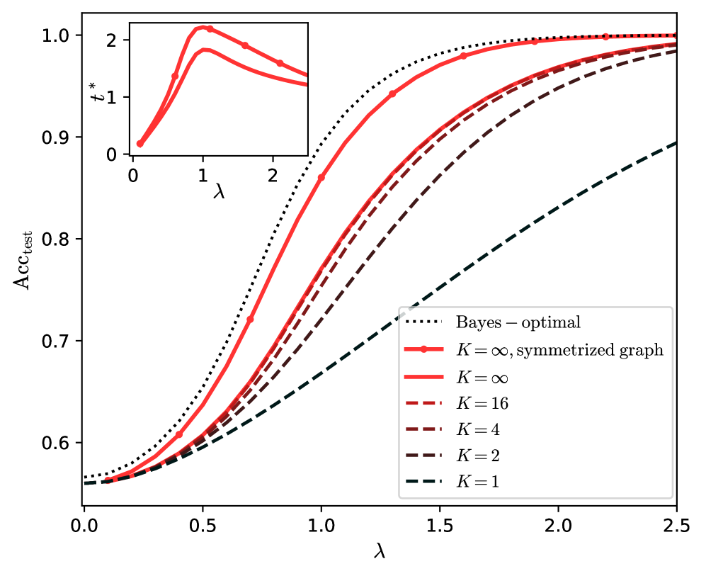
\n ## Chart: Test Accuracy vs. Lambda ### Overview The image presents a line chart illustrating the relationship between a parameter lambda (λ) and the test accuracy (Acc_test) for different values of K. A smaller inset chart shows the relationship between lambda and t*. The chart appears to be evaluating the performance of a model or algorithm under varying conditions. ### Components/Axes * **X-axis:** Lambda (λ), ranging from 0.0 to 2.5. * **Y-axis:** Test Accuracy (Acc_test), ranging from 0.55 to 1.05. * **Inset Chart X-axis:** Lambda (λ), ranging from 0.0 to 2.5. * **Inset Chart Y-axis:** t*, ranging from 0.0 to 2.5. * **Legend:** Located in the top-right corner, listing the different lines: * Bayes – optimal (solid blue line) * K = ∞, symmetrized graph (dotted red line) * K = ∞ (solid red line) * K = 16 (dashed brown line) * K = 4 (dashed dark red line) * K = 2 (dashed black line) * K = 1 (dashed very dark black line) ### Detailed Analysis The main chart displays several lines representing different values of K. * **Bayes – optimal (solid blue line):** This line starts at approximately 0.62 at λ = 0.0, rises rapidly to approximately 0.95 at λ = 0.7, and then plateaus, remaining around 0.98-1.0 for λ > 1.0. * **K = ∞, symmetrized graph (dotted red line):** This line begins at approximately 0.62 at λ = 0.0, increases steadily to approximately 0.95 at λ = 1.0, and then plateaus around 0.98-1.0 for λ > 1.0. * **K = ∞ (solid red line):** This line starts at approximately 0.62 at λ = 0.0, rises steadily to approximately 0.95 at λ = 1.0, and then plateaus around 0.98-1.0 for λ > 1.0. * **K = 16 (dashed brown line):** This line starts at approximately 0.62 at λ = 0.0, increases more slowly than the previous lines, reaching approximately 0.85 at λ = 1.0, and then continues to rise, approaching 0.95 at λ = 2.5. * **K = 4 (dashed dark red line):** This line starts at approximately 0.62 at λ = 0.0, increases slowly, reaching approximately 0.75 at λ = 1.0, and then continues to rise, approaching 0.90 at λ = 2.5. * **K = 2 (dashed black line):** This line starts at approximately 0.62 at λ = 0.0, increases very slowly, reaching approximately 0.68 at λ = 1.0, and then continues to rise, approaching 0.80 at λ = 2.5. * **K = 1 (dashed very dark black line):** This line starts at approximately 0.62 at λ = 0.0, increases extremely slowly, reaching approximately 0.65 at λ = 1.0, and then continues to rise, approaching 0.75 at λ = 2.5. The inset chart shows a curve for t* vs. λ. The curve peaks at approximately t* = 2.1 at λ = 0.8, and then decreases to approximately t* = 1.0 at λ = 2.5. ### Key Observations * The "Bayes – optimal" and "K = ∞" lines achieve the highest test accuracy, plateauing around 0.98-1.0 for λ > 1.0. * As K decreases, the test accuracy decreases, and the rate of increase with respect to λ slows down. * The inset chart shows a non-monotonic relationship between t* and λ, with a peak around λ = 0.8. * All lines start at the same accuracy level (approximately 0.62) when λ = 0. ### Interpretation The chart demonstrates the impact of the parameter K on the test accuracy of a model as a function of lambda (λ). The "Bayes – optimal" line represents the theoretical upper bound on performance. The lines corresponding to higher values of K (K = ∞ and K = 16) approach this optimal performance more closely than those with lower values of K (K = 4, K = 2, and K = 1). This suggests that increasing K improves the model's ability to generalize to unseen data, up to a certain point. The inset chart provides additional information about a parameter t* that is related to λ. The peak in the curve suggests that there is an optimal value of λ (around 0.8) that maximizes t*. The relationship between t* and λ may be indicative of the model's sensitivity to changes in λ. The data suggests that for achieving high test accuracy, a larger value of K is preferable, and that there is a specific value of lambda that optimizes another parameter, t*. The choice of K and λ should be made based on the desired trade-off between accuracy and other factors, such as computational cost or model complexity.

\n ## Line Chart with Inset: Test Accuracy vs. Lambda for Different K Values ### Overview The image is a technical line chart illustrating the relationship between a parameter `λ` (lambda) and test accuracy (`Acc_test`) for various model configurations, characterized by a parameter `K`. The chart includes a primary plot and a smaller inset plot. The primary plot shows multiple curves converging towards high accuracy as `λ` increases. The inset plot shows the behavior of a variable `t*` against `λ`. ### Components/Axes **Main Chart:** * **Y-axis:** Label is `Acc_test`. Scale ranges from approximately 0.55 to 1.0, with major ticks at 0.6, 0.7, 0.8, 0.9, and 1.0. * **X-axis:** Label is `λ`. Scale ranges from 0.0 to 2.5, with major ticks at 0.0, 0.5, 1.0, 1.5, 2.0, and 2.5. * **Legend:** Located in the bottom-right quadrant of the main chart area. It contains seven entries, each associating a line style/color with a model configuration. 1. `Bayes – optimal`: Black dotted line. 2. `K = ∞, symmetrized graph`: Solid red line with circular markers. 3. `K = ∞`: Solid red line (no markers). 4. `K = 16`: Dashed red line. 5. `K = 4`: Dash-dot dark red/brown line. 6. `K = 2`: Dashed dark red/brown line. 7. `K = 1`: Dashed dark gray/black line. **Inset Chart (Top-Left Corner):** * **Y-axis:** Label is `t*`. Scale shows ticks at 0, 1, and 2. * **X-axis:** Label is `λ`. Scale shows ticks at 0, 1, and 2. * **Content:** Contains two solid red lines (one slightly thicker than the other) plotting `t*` against `λ`. ### Detailed Analysis **Main Chart Trends & Approximate Data Points:** All curves show a sigmoidal (S-shaped) increase in test accuracy as `λ` increases from 0.0 to approximately 2.0, after which they plateau. 1. **Bayes – optimal (Black Dotted):** This is the upper bound. It starts at ~0.56 accuracy at λ=0.0, rises steeply, and approaches 1.0 accuracy by λ≈1.5. 2. **K = ∞, symmetrized graph (Solid Red with Markers):** This is the best-performing practical model. It closely follows the Bayes-optimal curve but is slightly below it. It starts at ~0.555 at λ=0.0, crosses 0.9 accuracy around λ≈1.0, and converges to near 1.0 by λ≈2.0. 3. **K = ∞ (Solid Red):** Performs slightly worse than the symmetrized version. It starts at a similar point (~0.555) but remains below the symmetrized curve across the entire range. 4. **K = 16 (Dashed Red):** Starts at ~0.555. Its rise is less steep than the K=∞ curves. It reaches 0.9 accuracy around λ≈1.3 and approaches but does not fully reach 1.0 by λ=2.5. 5. **K = 4 (Dash-Dot Dark Red):** Starts at ~0.555. Its slope is shallower. It reaches 0.8 accuracy around λ≈1.2 and is at ~0.97 by λ=2.5. 6. **K = 2 (Dashed Dark Red):** Starts at ~0.555. Its rise is even more gradual. It reaches 0.8 accuracy around λ≈1.6 and is at ~0.95 by λ=2.5. 7. **K = 1 (Dashed Dark Gray):** This is the lowest-performing curve. It starts at ~0.555 and increases almost linearly with a shallow slope, reaching only ~0.90 accuracy by λ=2.5. **Inset Chart Trends:** The two red lines in the inset show that `t*` initially increases with `λ`, peaks at a value slightly above 2 when `λ` is around 1.0, and then gradually decreases as `λ` increases further towards 2.0. ### Key Observations 1. **Performance Hierarchy:** There is a clear and consistent hierarchy: Bayes-optimal > K=∞, symmetrized > K=∞ > K=16 > K=4 > K=2 > K=1. This demonstrates that increasing the parameter `K` leads to higher test accuracy for a given `λ`. 2. **Convergence:** All models except K=1 show strong convergence towards the Bayes-optimal performance as `λ` increases, though the rate of convergence slows dramatically for lower `K` values. 3. **Symmetrization Benefit:** The "symmetrized graph" variant of K=∞ provides a small but consistent accuracy improvement over the standard K=∞ model across the entire `λ` range. 4. **Inset Peak:** The variable `t*` exhibits a non-monotonic relationship with `λ`, suggesting an optimal `λ` value (around 1.0) for maximizing `t*`. ### Interpretation This chart likely comes from a study on graph-based semi-supervised learning or a similar field where `K` represents the number of neighbors or a graph connectivity parameter, and `λ` controls the influence of the graph structure or a regularization term. * **What the data suggests:** The results demonstrate that richer graph structures (higher `K`) enable models to more effectively leverage the parameter `λ` to approach theoretical optimal (Bayesian) performance. The symmetrization of the graph provides an additional, modest boost, likely by enforcing a more robust similarity measure. * **Relationship between elements:** The main chart and inset are linked by the common x-axis variable `λ`. The peak in `t*` at `λ≈1.0` in the inset may correspond to the region in the main chart where the accuracy curves begin their steepest ascent, suggesting `t*` could be a measure of training dynamics, confidence, or another intermediate variable that is maximized at an intermediate regularization strength. * **Notable anomaly/trend:** The K=1 curve is a significant outlier in its poor performance and near-linear response. This implies that with minimal graph information (only self-connection or a trivial graph), the model's ability to improve with `λ` is severely hampered, and it cannot approach optimal performance within the plotted range. The chart argues strongly for using sufficiently large `K` in such models.

## Line Graph: Test Accuracy (Acc_test) vs. Regularization Parameter (λ) ### Overview The graph illustrates the relationship between the regularization parameter λ and test accuracy (Acc_test) for different model configurations. Multiple lines represent varying values of K (model complexity) and a Bayes-optimal baseline. An inset graph highlights behavior at lower λ values (0–2). ### Components/Axes - **X-axis (λ)**: Regularization parameter, ranging from 0 to 2.5. - **Y-axis (Acc_test)**: Test accuracy, ranging from 0.5 to 1.0. - **Legend**: - **Dotted black**: Bayes-optimal (upper bound). - **Solid red**: K = ∞, symmetrized graph. - **Dashed red**: K = 16. - **Dotted red**: K = 4. - **Dashed brown**: K = 2. - **Dotted green**: K = 1. ### Detailed Analysis 1. **Bayes-optimal (dotted black)**: - Remains flat at Acc_test ≈ 1.0 across all λ. - Serves as the theoretical maximum accuracy. 2. **K = ∞, symmetrized graph (solid red)**: - Stays nearly parallel to the Bayes-optimal line, with Acc_test ≈ 0.98–1.0. - Minimal deviation suggests near-optimal performance. 3. **K = 16 (dashed red)**: - Acc_test increases from ~0.55 (λ=0) to ~0.95 (λ=2.5). - Slightly lags behind K = ∞ but converges at higher λ. 4. **K = 4 (dotted red)**: - Acc_test rises from ~0.52 (λ=0) to ~0.88 (λ=2.5). - Shows a steeper initial increase but plateaus earlier. 5. **K = 2 (dashed brown)**: - Acc_test climbs from ~0.50 (λ=0) to ~0.82 (λ=2.5). - Slower growth compared to higher K values. 6. **K = 1 (dotted green)**: - Acc_test increases from ~0.48 (λ=0) to ~0.75 (λ=2.5). - Lowest performance, indicating underfitting. 7. **Inset Graph (λ=0–2)**: - Zooms into the lower λ range, showing a peak at λ ≈ 1 for K = ∞ and K = 16. - Lines for K = 4, 2, and 1 intersect near λ = 1, suggesting a critical transition point. ### Key Observations - **Trend Verification**: - All lines exhibit upward trends as λ increases, confirming that regularization improves performance. - Higher K values (e.g., K = ∞, 16) achieve higher Acc_test, aligning with expectations for model complexity. - The inset reveals a local maximum at λ ≈ 1 for K = ∞ and K = 16, followed by a slight decline before stabilization. - **Legend Consistency**: - Colors and line styles match the legend exactly (e.g., solid red for K = ∞, dashed red for K = 16). ### Interpretation The graph demonstrates that: 1. **Model Complexity (K)**: Higher K values (e.g., K = ∞) achieve near-optimal accuracy, while lower K values (e.g., K = 1) underperform due to underfitting. 2. **Regularization Impact**: Increasing λ improves test accuracy across all K values, but the rate of improvement depends on K. Higher K models benefit more from regularization. 3. **Optimal λ**: The inset suggests λ ≈ 1 may be optimal for K = ∞ and K = 16, though performance stabilizes at higher λ. For lower K values, the optimal λ is less distinct but still critical for balancing bias-variance trade-offs. 4. **Bayes-optimal Baseline**: The flat dotted black line underscores the theoretical limit, emphasizing that practical models (even with K = ∞) cannot exceed this bound. This analysis highlights the interplay between model complexity, regularization, and performance, providing insights for tuning λ and K in machine learning pipelines.