\n
## Line Chart with Inset: Test Accuracy vs. Lambda for Different K Values
### Overview
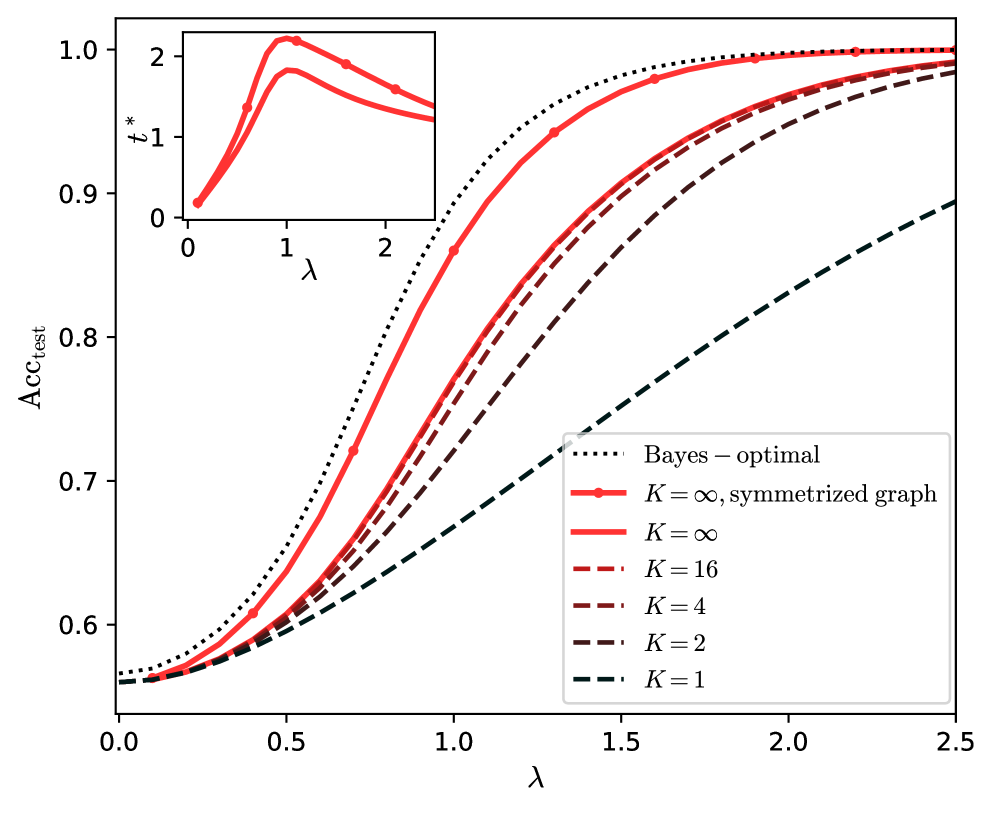
The image is a technical line chart illustrating the relationship between a parameter `λ` (lambda) and test accuracy (`Acc_test`) for various model configurations, characterized by a parameter `K`. The chart includes a primary plot and a smaller inset plot. The primary plot shows multiple curves converging towards high accuracy as `λ` increases. The inset plot shows the behavior of a variable `t*` against `λ`.
### Components/Axes
**Main Chart:**
* **Y-axis:** Label is `Acc_test`. Scale ranges from approximately 0.55 to 1.0, with major ticks at 0.6, 0.7, 0.8, 0.9, and 1.0.
* **X-axis:** Label is `λ`. Scale ranges from 0.0 to 2.5, with major ticks at 0.0, 0.5, 1.0, 1.5, 2.0, and 2.5.
* **Legend:** Located in the bottom-right quadrant of the main chart area. It contains seven entries, each associating a line style/color with a model configuration.
1. `Bayes – optimal`: Black dotted line.
2. `K = ∞, symmetrized graph`: Solid red line with circular markers.
3. `K = ∞`: Solid red line (no markers).
4. `K = 16`: Dashed red line.
5. `K = 4`: Dash-dot dark red/brown line.
6. `K = 2`: Dashed dark red/brown line.
7. `K = 1`: Dashed dark gray/black line.
**Inset Chart (Top-Left Corner):**
* **Y-axis:** Label is `t*`. Scale shows ticks at 0, 1, and 2.
* **X-axis:** Label is `λ`. Scale shows ticks at 0, 1, and 2.
* **Content:** Contains two solid red lines (one slightly thicker than the other) plotting `t*` against `λ`.
### Detailed Analysis
**Main Chart Trends & Approximate Data Points:**
All curves show a sigmoidal (S-shaped) increase in test accuracy as `λ` increases from 0.0 to approximately 2.0, after which they plateau.
1. **Bayes – optimal (Black Dotted):** This is the upper bound. It starts at ~0.56 accuracy at λ=0.0, rises steeply, and approaches 1.0 accuracy by λ≈1.5.
2. **K = ∞, symmetrized graph (Solid Red with Markers):** This is the best-performing practical model. It closely follows the Bayes-optimal curve but is slightly below it. It starts at ~0.555 at λ=0.0, crosses 0.9 accuracy around λ≈1.0, and converges to near 1.0 by λ≈2.0.
3. **K = ∞ (Solid Red):** Performs slightly worse than the symmetrized version. It starts at a similar point (~0.555) but remains below the symmetrized curve across the entire range.
4. **K = 16 (Dashed Red):** Starts at ~0.555. Its rise is less steep than the K=∞ curves. It reaches 0.9 accuracy around λ≈1.3 and approaches but does not fully reach 1.0 by λ=2.5.
5. **K = 4 (Dash-Dot Dark Red):** Starts at ~0.555. Its slope is shallower. It reaches 0.8 accuracy around λ≈1.2 and is at ~0.97 by λ=2.5.
6. **K = 2 (Dashed Dark Red):** Starts at ~0.555. Its rise is even more gradual. It reaches 0.8 accuracy around λ≈1.6 and is at ~0.95 by λ=2.5.
7. **K = 1 (Dashed Dark Gray):** This is the lowest-performing curve. It starts at ~0.555 and increases almost linearly with a shallow slope, reaching only ~0.90 accuracy by λ=2.5.
**Inset Chart Trends:**
The two red lines in the inset show that `t*` initially increases with `λ`, peaks at a value slightly above 2 when `λ` is around 1.0, and then gradually decreases as `λ` increases further towards 2.0.
### Key Observations
1. **Performance Hierarchy:** There is a clear and consistent hierarchy: Bayes-optimal > K=∞, symmetrized > K=∞ > K=16 > K=4 > K=2 > K=1. This demonstrates that increasing the parameter `K` leads to higher test accuracy for a given `λ`.
2. **Convergence:** All models except K=1 show strong convergence towards the Bayes-optimal performance as `λ` increases, though the rate of convergence slows dramatically for lower `K` values.
3. **Symmetrization Benefit:** The "symmetrized graph" variant of K=∞ provides a small but consistent accuracy improvement over the standard K=∞ model across the entire `λ` range.
4. **Inset Peak:** The variable `t*` exhibits a non-monotonic relationship with `λ`, suggesting an optimal `λ` value (around 1.0) for maximizing `t*`.
### Interpretation
This chart likely comes from a study on graph-based semi-supervised learning or a similar field where `K` represents the number of neighbors or a graph connectivity parameter, and `λ` controls the influence of the graph structure or a regularization term.
* **What the data suggests:** The results demonstrate that richer graph structures (higher `K`) enable models to more effectively leverage the parameter `λ` to approach theoretical optimal (Bayesian) performance. The symmetrization of the graph provides an additional, modest boost, likely by enforcing a more robust similarity measure.
* **Relationship between elements:** The main chart and inset are linked by the common x-axis variable `λ`. The peak in `t*` at `λ≈1.0` in the inset may correspond to the region in the main chart where the accuracy curves begin their steepest ascent, suggesting `t*` could be a measure of training dynamics, confidence, or another intermediate variable that is maximized at an intermediate regularization strength.
* **Notable anomaly/trend:** The K=1 curve is a significant outlier in its poor performance and near-linear response. This implies that with minimal graph information (only self-connection or a trivial graph), the model's ability to improve with `λ` is severely hampered, and it cannot approach optimal performance within the plotted range. The chart argues strongly for using sufficiently large `K` in such models.