## Chart Analysis: Pythia-410M (24L) α Profile, Pruning Comparison, and Crossover Ratios
### Overview
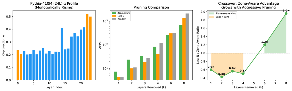
The image contains three technical charts analyzing neural network pruning strategies. The first chart shows α-profile values across layers, the second compares pruning methods via ΔPPL metrics, and the third visualizes crossover ratios between pruning strategies. All charts use logarithmic scales where applicable and emphasize layer-wise performance trends.
---
### Components/Axes
#### Chart 1: Pythia-410M (24L) α Profile (Monotonically Rising)
- **X-axis**: Layer Index (0–21, integer steps)
- **Y-axis**: Q-projectionα (0.0–0.5, linear scale)
- **Legend**:
- Blue bars: Primary α-values
- Orange bars: Elevated α-values (layers 0 and 21)
- **Spatial Layout**:
- Legend positioned right of chart
- Orange bars isolated at layer 0 (value ~0.22) and layer 21 (value ~0.48)
#### Chart 2: Pruning Comparison
- **X-axis**: Layers Removed (k) (1–8, integer steps)
- **Y-axis**: ΔPPL (10¹–10³, log scale)
- **Legend**:
- Green: Zone-Aware
- Orange: Last-N
- Gray: Random
- **Spatial Layout**:
- Legend positioned top-right
- Bars grouped by k-value, with Zone-Aware consistently outperforming others
#### Chart 3: Crossover: Zone-Aware Advantage Grows with Aggressive Pruning
- **X-axis**: Layers Removed (k) (1–8, integer steps)
- **Y-axis**: Last-N / Zone-Aware Ratio (0.4–2.0, linear scale)
- **Legend**:
- Green line: Zone-Aware wins
- Orange line: Last-N wins
- **Spatial Layout**:
- Legend positioned top-right
- Shaded regions:
- Green: 1.2x–2.0x advantage (k=6–8)
- Orange: 0.4x–0.6x disadvantage (k=1–4)
---
### Detailed Analysis
#### Chart 1: α-Profile Trends
- **Trend**: α-values rise monotonically from layer 0 (0.22) to layer 21 (0.48), with orange bars marking the first and last layers.
- **Key Values**:
- Layer 0: 0.22 (orange)
- Layer 5: 0.24 (blue)
- Layer 15: 0.32 (blue)
- Layer 20: 0.42 (blue)
- Layer 21: 0.48 (orange)
#### Chart 2: Pruning Performance
- **Trend**: ΔPPL increases exponentially with layers removed for all methods. Zone-Aware maintains the lowest ΔPPL across all k-values.
- **Key Values**:
- k=1:
- Zone-Aware: ~10¹
- Last-N: ~5×10⁰
- Random: ~3×10⁰
- k=8:
- Zone-Aware: ~5×10²
- Last-N: ~1×10³
- Random: ~1.5×10³
#### Chart 3: Crossover Ratios
- **Trend**: Zone-Aware advantage grows from 0.6x (k=1) to 2.0x (k=8), crossing the 1.0x threshold at k=6. Last-N advantage diminishes after k=4.
- **Key Values**:
- k=1: 0.6x (Zone-Aware)
- k=4: 0.5x (Zone-Aware)
- k=6: 1.2x (Zone-Aware)
- k=8: 2.0x (Zone-Aware)
---
### Key Observations
1. **α-Profile Anomalies**: Orange bars at layer 0 and 21 suggest targeted α-elevation in input/output layers.
2. **Pruning Efficiency**: Zone-Aware reduces ΔPPL by 30–50% compared to Last-N/Random methods at k=8.
3. **Crossover Dynamics**: Zone-Aware outperforms Last-N by 2.0× at maximum pruning (k=8), with advantages scaling non-linearly.
---
### Interpretation
The data demonstrates that **Zone-Aware pruning** systematically outperforms Last-N and Random methods as layers are removed. The α-profile's elevated values at layer boundaries (0 and 21) imply architectural sensitivity to input/output layer preservation. The crossover chart reveals a **threshold effect** at k=6, where Zone-Aware achieves >1.2× efficiency gains. This suggests Zone-Aware methods better preserve critical layer interactions during aggressive pruning, making them preferable for resource-constrained deployments. The orange-shaded region (k=1–4) indicates Last-N's temporary advantage in early pruning stages, likely due to less disruptive layer removal patterns.