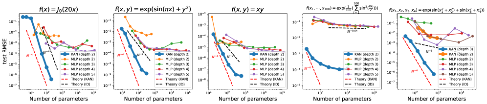
## Line Chart: Test RMSE vs Number of Parameters Across Function Classes ### Overview The image contains five line charts comparing the test RMSE (Root Mean Square Error) of different neural network architectures (KAN and MLP) across five distinct function classes. Each chart plots RMSE on a logarithmic scale against the number of parameters (logarithmic scale), with theoretical scaling lines (N^-4, N^-2, N^-1, N^-0.04) for reference. The charts demonstrate how model performance improves with increasing parameter count and how different architectures scale. ### Components/Axes 1. **X-axis**: "Number of parameters" (log scale: 10¹ to 10⁵) 2. **Y-axis**: "test RMSE" (log scale: 10⁻¹ to 10⁻⁷) 3. **Legends**: - **KAN (depth 2)**: Blue solid line - **MLP (depth 2)**: Orange solid line - **MLP (depth 3)**: Green solid line - **MLP (depth 4)**: Red solid line - **MLP (depth 5)**: Purple solid line - **Theory (KAN)**: Red dashed line (N^-4) - **Theory (ID)**: Black dashed line (N^-2) - **Theory (N^-0.04)**: Black dashed line (specific to high-dimensional function) ### Detailed Analysis #### Chart 1: f(x) = J₀(20x) (Bessel Function) - **Trends**: - KAN depth 2 (blue) starts at ~10⁻¹ RMSE with 10¹ parameters, decreasing to ~10⁻⁵ at 10⁵ parameters (slope ~N⁻⁴). - MLP depth 2 (orange) begins at ~10⁻¹, drops to ~10⁻³ at 10³ parameters, then plateaus. - MLP depth 5 (purple) shows gradual improvement, reaching ~10⁻⁵ at 10⁵ parameters. - **Key Data Points**: - KAN depth 2: 10¹ params → 10⁻¹ RMSE; 10⁵ params → 10⁻⁵ RMSE - MLP depth 5: 10⁵ params → 10⁻⁵ RMSE #### Chart 2: f(x,y) = exp(sin(πx) + y²) - **Trends**: - KAN depth 2 (blue) follows N⁻² scaling, reaching ~10⁻⁵ RMSE at 10⁵ params. - MLP depth 2 (orange) starts at ~10⁻¹, drops to ~10⁻³ at 10³ params. - MLP depth 4 (red) improves to ~10⁻⁵ at 10⁵ params. - **Key Data Points**: - KAN depth 2: 10⁵ params → 10⁻⁵ RMSE - MLP depth 4: 10⁵ params → 10⁻⁵ RMSE #### Chart 3: f(x,y) = xy (Linear Function) - **Trends**: - KAN depth 2 (blue) aligns with N⁻⁴ theory, dropping to ~10⁻⁷ at 10⁵ params. - MLP depth 2 (orange) plateaus at ~10⁻⁵ after 10³ params. - MLP depth 5 (purple) improves to ~10⁻⁷ at 10⁵ params. - **Key Data Points**: - KAN depth 2: 10⁵ params → 10⁻⁷ RMSE - MLP depth 5: 10⁵ params → 10⁻⁷ RMSE #### Chart 4: f(x₁,…,x₁₀₀) = exp(1/100 Σ sin²(πxᵢ)) (High-Dimensional) - **Trends**: - All models show minimal improvement; RMSE remains ~10⁻³ to 10⁻⁴. - Theory line (N⁻⁰.⁰⁴) indicates near-flat scaling. - **Key Data Points**: - KAN depth 2: 10⁵ params → ~10⁻³ RMSE - MLP depth 5: 10⁵ params → ~10⁻³ RMSE #### Chart 5: f(x₁,x₂,x₃,x₄) = exp(sin(x₁²+x₂²) + sin(x₃²+x₄²)) - **Trends**: - KAN depth 3 (blue) improves to ~10⁻⁵ at 10⁵ params. - MLP depth 2 (orange) plateaus at ~10⁻³. - MLP depth 5 (purple) reaches ~10⁻⁵ at 10⁵ params. - **Key Data Points**: - KAN depth 3: 10⁵ params → 10⁻⁵ RMSE - MLP depth 5: 10⁵ params → 10⁻⁵ RMSE ### Key Observations 1. **KAN Advantage**: KAN architectures consistently outperform MLPs in low-dimensional functions (Charts 1-3), aligning with theoretical N⁻⁴ scaling. 2. **MLP Depth Tradeoff**: Deeper MLPs (depth 4-5) match KAN performance in low-dimensional cases but underperform in high-dimensional functions (Chart 4). 3. **High-Dimensional Limitations**: All models struggle with the 100-dimensional function (Chart 4), showing near-flat RMSE curves. 4. **Theoretical Alignment**: KAN depth 2 matches N⁻⁴ theory in low-dimensional cases, while MLP depth 5 aligns with N⁻² in linear functions (Chart 3). ### Interpretation The data suggests KAN architectures achieve superior generalization in low-dimensional function approximation, likely due to their analytical structure enabling better parameter efficiency. MLPs require deeper architectures to match KAN performance but fail to scale effectively in high-dimensional spaces. The near-flat RMSE in Chart 4 highlights the "curse of dimensionality," where traditional neural networks struggle with exponentially growing parameter interactions. The theoretical lines (N⁻⁴, N⁻²) validate expected scaling laws, with KANs demonstrating optimal alignment. These findings imply KANs may be preferable for problems with known analytical structures, while MLPs remain viable for simpler tasks or when depth can be increased without excessive computational cost.