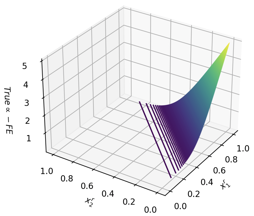
## 3D Surface Plot: True α - FE vs. x₁' and x₂'
### Overview
The image displays a three-dimensional surface plot rendered within a wireframe box. The plot visualizes a mathematical function where a dependent variable, labeled "True α - FE", is plotted against two independent variables, "x₁'" and "x₂'". The surface exhibits a pronounced, smooth curvature, rising from a low value near the origin to a high peak at the opposite corner of the domain.
### Components/Axes
* **Vertical Axis (Z-axis):**
* **Label:** "True α - FE"
* **Scale:** Linear, ranging from 1 to 5. Major tick marks are present at integer intervals (1, 2, 3, 4, 5).
* **Horizontal Axis 1 (X-axis, front-left):**
* **Label:** "x₂'"
* **Scale:** Linear, ranging from 0.0 to 1.0. Major tick marks are at 0.0, 0.2, 0.4, 0.6, 0.8, 1.0.
* **Horizontal Axis 2 (Y-axis, front-right):**
* **Label:** "x₁'"
* **Scale:** Linear, ranging from 0.0 to 1.0. Major tick marks are at 0.0, 0.2, 0.4, 0.6, 0.8, 1.0.
* **Plot Area:** A 3D wireframe box defines the plotting volume. The surface is rendered as a continuous, colored mesh.
* **Color Mapping:** The surface color is mapped to the vertical axis ("True α - FE") value. The gradient runs from dark purple (low values, ~1) through blue and green to bright yellow (high values, >5).
### Detailed Analysis
* **Surface Shape and Trend:** The surface forms a smooth, upward-curving sheet. It is lowest near the corner where both x₁' and x₂' are 0.0. From there, it slopes upward with increasing steepness as both x₁' and x₂' increase. The maximum value occurs at the corner where x₁' = 1.0 and x₂' = 1.0.
* **Data Point Extraction (Approximate):**
* At (x₁' ≈ 0.0, x₂' ≈ 0.0): True α - FE ≈ 1.0 (dark purple region).
* At (x₁' ≈ 0.5, x₂' ≈ 0.5): True α - FE ≈ 2.0 - 2.5 (blue region).
* At (x₁' ≈ 1.0, x₂' ≈ 0.0): True α - FE ≈ 1.5 - 2.0 (purple-blue region).
* At (x₁' ≈ 0.0, x₂' ≈ 1.0): True α - FE ≈ 1.5 - 2.0 (purple-blue region).
* At (x₁' ≈ 1.0, x₂' ≈ 1.0): True α - FE > 5.0 (bright yellow peak). The surface extends beyond the top of the defined axis range at this point.
* **Spatial Grounding:** The legend (color bar) is implicit, mapped directly to the Z-axis. The highest point (yellow) is spatially located at the top-right-back corner of the 3D box, corresponding to the maximum values of both input variables. The lowest points (dark purple) are along the edges where at least one input variable is near 0.0.
### Key Observations
1. **Exponential-like Growth:** The relationship is highly non-linear. The increase in "True α - FE" accelerates dramatically as both x₁' and x₂' approach 1.0.
2. **Symmetry:** The surface appears roughly symmetric with respect to the x₁' = x₂' diagonal. The values along the line where x₁' = x₂' are higher than points where the variables are unequal but have the same average.
3. **Domain Coverage:** The plotted surface does not cover the entire [0,1] x [0,1] domain. It is absent from the region where x₁' is low and x₂' is high, and vice-versa, suggesting the function may be undefined or zero in those areas, or the plot is intentionally clipped.
4. **Color as Data:** The color gradient provides a strong visual cue for the magnitude of the Z-value, reinforcing the spatial trend.
### Interpretation
This plot likely represents the output of a mathematical model or simulation where the quantity "True α - FE" is a function of two normalized parameters, x₁' and x₂'. The steep, convex curvature suggests a synergistic or multiplicative interaction between the two parameters; their combined effect is greater than the sum of their individual effects.
The fact that the peak exceeds the charted Z-axis limit (5) indicates the function's value grows very rapidly in the corner of the parameter space. This could model phenomena like reaction rates, error surfaces in optimization, or sensitivity analyses where certain parameter combinations lead to extreme outcomes. The absence of the surface in parts of the domain might indicate physical constraints, regions of instability, or simply the chosen viewing angle and clipping plane of the 3D renderer. The plot effectively communicates that to maximize "True α - FE," both input parameters must be pushed to their upper limit values simultaneously, i.e., 1.0 and 1.0.