## Chart: Energy vs. Time for Different Network Topologies
### Overview
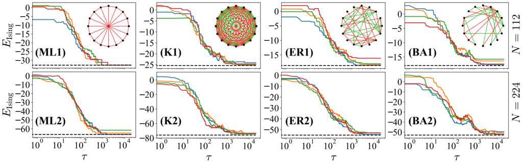
The image presents a series of line graphs showing the relationship between energy (E_Ising) and time (τ) for different network topologies. There are eight subplots arranged in a 2x4 grid. Each subplot corresponds to a specific network topology (ML, K, ER, BA) and network size (N=112 or N=224). Each subplot also contains a small network diagram illustrating the network topology. The x-axis (τ) is on a logarithmic scale. Each graph contains four lines, but the legend is missing.
### Components/Axes
* **Y-axis (Vertical):** E_Ising (Energy), with a range from approximately 0 to -30 for N=112 and 0 to -60 or -80 for N=224.
* Y-axis markers: 0, -5, -10, -15, -20, -25, -30 (for top row); 0, -10, -20, -30, -40, -50, -60 (for bottom row, except K2 which goes to -80).
* **X-axis (Horizontal):** τ (Time), logarithmic scale from 10^0 to 10^4.
* X-axis markers: 10^0, 10^1, 10^2, 10^3, 10^4.
* **Subplot Titles:** (ML1), (K1), (ER1), (BA1) for the top row and (ML2), (K2), (ER2), (BA2) for the bottom row.
* **Network Size Labels:** N = 112 (right of the top row), N = 224 (right of the bottom row).
* **Network Diagrams:** Small diagrams within each subplot illustrating the network topology.
* **Horizontal Dashed Line:** A horizontal dashed line is present in each subplot, representing a baseline energy level.
### Detailed Analysis
**General Trend:**
All plots show a general downward trend, indicating that the energy decreases as time increases. The rate of decrease varies depending on the network topology and size.
**Subplot-Specific Analysis:**
* **(ML1):** N=112, Topology: ML. The four lines (blue, red, green, orange) start near 0 and decrease to approximately -30. The blue line appears to decrease slightly slower initially.
* **(K1):** N=112, Topology: K. The four lines (blue, red, green, orange) start near 0 and decrease to approximately -25. The blue line plateaus around -22.
* **(ER1):** N=112, Topology: ER. The four lines (blue, red, green, orange) start near 0 and decrease to approximately -16.
* **(BA1):** N=112, Topology: BA. The four lines (blue, red, green, orange) start near 0 and decrease to approximately -16.
* **(ML2):** N=224, Topology: ML. The four lines (blue, red, green, orange) start near 0 and decrease to approximately -60.
* **(K2):** N=224, Topology: K. The four lines (blue, red, green, orange) start near 0 and decrease to approximately -60.
* **(ER2):** N=224, Topology: ER. The four lines (blue, red, green, orange) start near 0 and decrease to approximately -50.
* **(BA2):** N=224, Topology: BA. The four lines (blue, red, green, orange) start near 0 and decrease to approximately -50.
**Network Topologies:**
* **ML:** Appears to be a mean-field like topology, with connections radiating from a central node.
* **K:** Appears to be a fully connected topology.
* **ER:** Appears to be an Erdos-Renyi random network.
* **BA:** Appears to be a Barabasi-Albert scale-free network.
### Key Observations
* The energy generally decreases as time increases for all network topologies and sizes.
* Increasing the network size (from N=112 to N=224) generally results in a lower final energy.
* The specific network topology influences the rate and extent of energy decrease.
* The dashed line represents the ground state energy.
### Interpretation
The plots illustrate the convergence of energy towards a ground state for different network topologies during some optimization process. The x-axis represents the time or iterations of the optimization. The different colored lines likely represent different initial conditions or parameters of the optimization algorithm. The network diagrams provide context for the underlying structure on which the optimization is performed. The data suggests that the network topology significantly impacts the efficiency and final energy state achieved during the optimization process. The larger networks (N=224) generally reach lower energy states, possibly due to the increased complexity and degrees of freedom. The different convergence rates for each topology suggest that some network structures are more amenable to this optimization process than others.