## Diagram: Graph Neural Network Processing Pipeline
### Overview
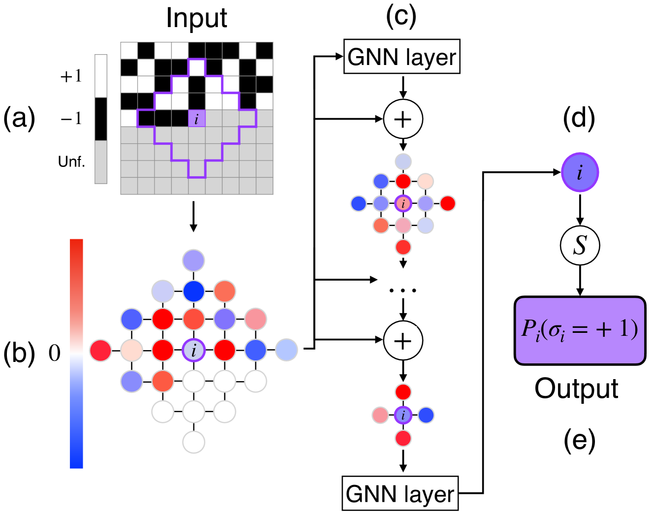
The diagram illustrates a multi-stage process for analyzing input data using graph neural networks (GNNs). It includes:
1. A binary input grid with labeled regions (+1, -1, Unf.)
2. A node-based representation with color-coded values
3. GNN layers processing node interactions
4. A probabilistic output for node classification
### Components/Axes
#### (a) Input Grid
- **Legend**:
- `+1` (white squares)
- `-1` (black squares)
- `Unf.` (gray squares)
- **Spatial Features**:
- Purple outline highlights a specific region (centered on node `i`)
- Grid dimensions: 8x8 squares (approximate)
#### (b) Node Representation
- **Color Gradient**:
- Red → Blue scale (0 → 1)
- Node `i` marked with purple outline
- **Connections**:
- Nodes linked in a hierarchical structure (top-down aggregation)
#### (c) GNN Layer 1
- **Structure**:
- Nodes colored in red, blue, and purple (matching gradient in (b))
- Central node `i` (purple) with weighted connections
- **Operation**:
- Summation (`+`) of node features
#### (d) Probabilistic Output
- **Equation**:
- `P_i(σ_i = +1)` (probability of node `i` being +1)
- **Symbol**:
- `S` (likely a sigmoid or softmax function)
#### (e) GNN Layer 2
- **Structure**:
- Simplified node network with fewer connections
- Node `i` retains central position
### Detailed Analysis
#### (a) Input Grid
- Binary classification (`+1`/`-1`) with undefined regions (`Unf.`).
- Purple outline suggests a focus on the central cluster of nodes.
#### (b) Node Representation
- Color gradient maps node values to a continuous scale (0–1).
- Node `i` (purple) likely represents a critical data point.
#### (c) GNN Layer 1
- Aggregates features from neighboring nodes (red/blue → purple).
- Central node `i` acts as a focal point for feature integration.
#### (d) Probabilistic Output
- Output `P_i(σ_i = +1)` quantifies confidence in node `i` being classified as `+1`.
#### (e) GNN Layer 2
- Simplifies the network while preserving node `i` as the target.
### Key Observations
1. **Input-Output Flow**:
- Input grid → Node embeddings → GNN processing → Probabilistic output.
2. **Node `i` Significance**:
- Highlighted in all stages, suggesting it is the primary target for analysis.
3. **Color Consistency**:
- Node colors in (b) and (c) align with the 0–1 gradient, ensuring accurate spatial grounding.
### Interpretation
This diagram models a GNN-based system for classifying nodes in a graph. The input grid (a) likely represents spatial or categorical data, where `+1`/`-1` denote binary labels and `Unf.` indicates missing/irrelevant data. The node network (b) transforms this input into embeddings, with node `i` as the focus. GNN layers (c, e) propagate and aggregate features, culminating in a probability output (d) that quantifies the likelihood of node `i` belonging to the `+1` class.
The use of color gradients and hierarchical node aggregation suggests the system handles both spatial relationships (via the grid) and graph-structured data (via GNNs). The purple outline in (a) and (b) emphasizes node `i`, indicating it may represent a critical entity (e.g., a user in a social network, a pixel in an image, or a sensor in IoT).
The absence of explicit numerical values for node features implies the diagram abstracts implementation details, focusing instead on the pipeline’s conceptual flow. The probabilistic output (d) aligns with common GNN applications like node classification or anomaly detection.