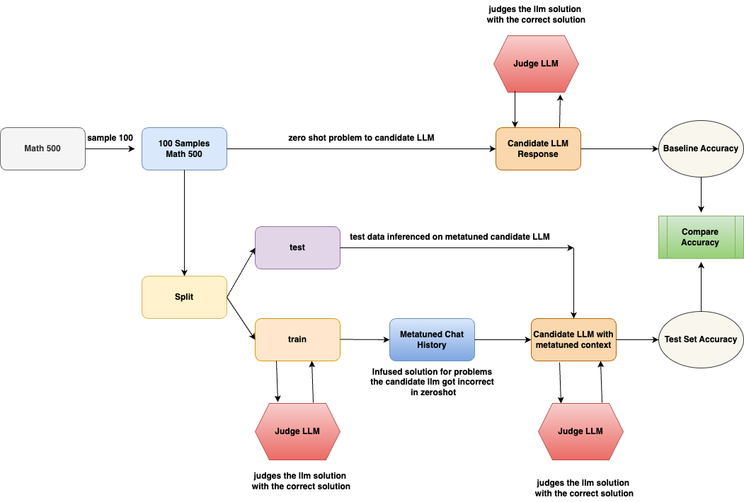
\n
## Flowchart: LLM Evaluation and Metatuning Process
### Overview
The image is a technical flowchart illustrating a two-path evaluation methodology for a Large Language Model (LLM). The process begins with a math problem dataset, samples it, and then evaluates a "Candidate LLM" under two conditions: a zero-shot baseline and a "metatuned" condition where the model is provided with context from its own past corrected errors. The final step compares the accuracy from both paths.
### Components/Axes
The diagram is structured as a directed graph with the following components, described from left to right, top to bottom:
**1. Initial Data Pipeline (Left Side):**
* **Math 500** (Gray rounded rectangle): The source dataset.
* **Arrow Label:** `sample 100`
* **100 Samples Math 500** (Light blue rounded rectangle): The sampled subset used for evaluation.
* **Split** (Yellow rounded rectangle): A process that divides the 100 samples into two subsets.
**2. Upper Path - Zero-Shot Evaluation:**
* **Arrow from "100 Samples Math 500":** Labeled `zero shot problem to candidate LLM`.
* **Candidate LLM Response** (Orange rounded rectangle): The output from the LLM when given a problem without prior examples.
* **Judge LLM** (Red hexagon, positioned above "Candidate LLM Response"): An external LLM that evaluates the candidate's response.
* **Annotation:** `judges the llm solution with the correct solution`
* **Baseline Accuracy** (Light gray oval): The accuracy metric derived from the zero-shot evaluation.
* **Arrow:** Points from "Candidate LLM Response" to "Baseline Accuracy".
**3. Lower Path - Metatuned Evaluation:**
* **From "Split":** Two arrows lead to:
* **test** (Light purple rounded rectangle): The test subset.
* **train** (Light orange rounded rectangle): The training subset.
* **From "train":**
* **Arrow to "Metatuned Chat History":** Labeled `infused solution for problems the candidate llm got incorrect in zeroshot`.
* **Judge LLM** (Red hexagon, positioned below "train"): Evaluates the training process.
* **Annotation:** `judges the llm solution with the correct solution`
* **Metatuned Chat History** (Blue rounded rectangle): A context window containing corrected solutions for problems the candidate LLM initially failed.
* **Candidate LLM with metatuned context** (Orange rounded rectangle): The same candidate LLM, now prompted with the "Metatuned Chat History" as context.
* **Arrow from "test":** Labeled `test data inferenced on metatuned candidate LLM`.
* **Judge LLM** (Red hexagon, positioned below "Candidate LLM with metatuned context"): Evaluates the metatuned model's output.
* **Annotation:** `judges the llm solution with the correct solution`
* **Test Set Accuracy** (Light gray oval): The accuracy metric from the metatuned evaluation.
**4. Final Comparison (Right Side):**
* **Compare Accuracy** (Green rectangle with vertical stripes): The final step that takes inputs from both "Baseline Accuracy" and "Test Set Accuracy".
* **Arrows:** One from "Baseline Accuracy" and one from "Test Set Accuracy" point into "Compare Accuracy".
### Detailed Analysis
The flowchart details a closed-loop system for LLM improvement and evaluation:
1. **Data Flow:** The process starts with 100 math problems. These are used in two parallel evaluations.
2. **Zero-Shot Path (Baseline):** The candidate LLM attempts all 100 problems without any examples. A separate "Judge LLM" grades these responses against correct solutions to establish a "Baseline Accuracy".
3. **Metatuned Path (Experimental):** The 100 samples are split. The "train" subset is used to create a "Metatuned Chat History". This history specifically contains the correct solutions for problems the candidate LLM got wrong in the zero-shot phase. This curated history is then used as context when the same LLM re-attempts the "test" subset of problems. The outputs are judged again to calculate "Test Set Accuracy".
4. **Evaluation:** A "Judge LLM" is used consistently in all three evaluation points (zero-shot response, training process, metatuned response) to ensure scoring consistency. Its role is explicitly defined each time.
5. **Goal:** The final "Compare Accuracy" block quantifies the performance difference between the baseline (zero-shot) and the enhanced (metatuned) model.
### Key Observations
* **Closed-Loop Learning:** The system is designed to learn from its own mistakes. The "Metatuned Chat History" is dynamically built from the model's zero-shot failures.
* **Role of Judge LLM:** The "Judge LLM" is a critical, recurring component, acting as an impartial grader separate from the candidate model being tested.
* **Spatial Layout:** The diagram uses a left-to-right flow for the main process, with the "Judge LLM" hexagons placed adjacent to the candidate LLM outputs they evaluate. The final comparison is isolated on the far right.
* **Color Coding:** Shapes are color-coded by function: gray for data, blue for processed data/history, orange for LLM states, yellow for processes, red for evaluation, and green for final analysis.
### Interpretation
This flowchart depicts a methodology for **meta-learning** or **self-improvement** in LLMs. The core hypothesis is that an LLM's performance on a task (here, math problems) can be improved by providing it with a context history that explicitly corrects its prior errors.
* **What it demonstrates:** It's a systematic approach to "teach" a model by showing it examples of its own mistakes and their corrections, then testing if this context improves its reasoning on new, similar problems. This is more targeted than general fine-tuning, as it uses the model's own failure modes as the training signal.
* **Relationships:** The "train" and "test" split is crucial. The model learns from corrections on the "train" set and is evaluated on unseen problems from the "test" set, preventing simple memorization. The "Judge LLM" provides an external, consistent metric for success.
* **Significance:** This process aims to answer: "Can an LLM become better at a task by being given a chat history that contains solutions to problems it previously failed?" The "Compare Accuracy" result would show the efficacy of this metatuning approach. The entire system is a framework for iterative, self-referential model improvement.