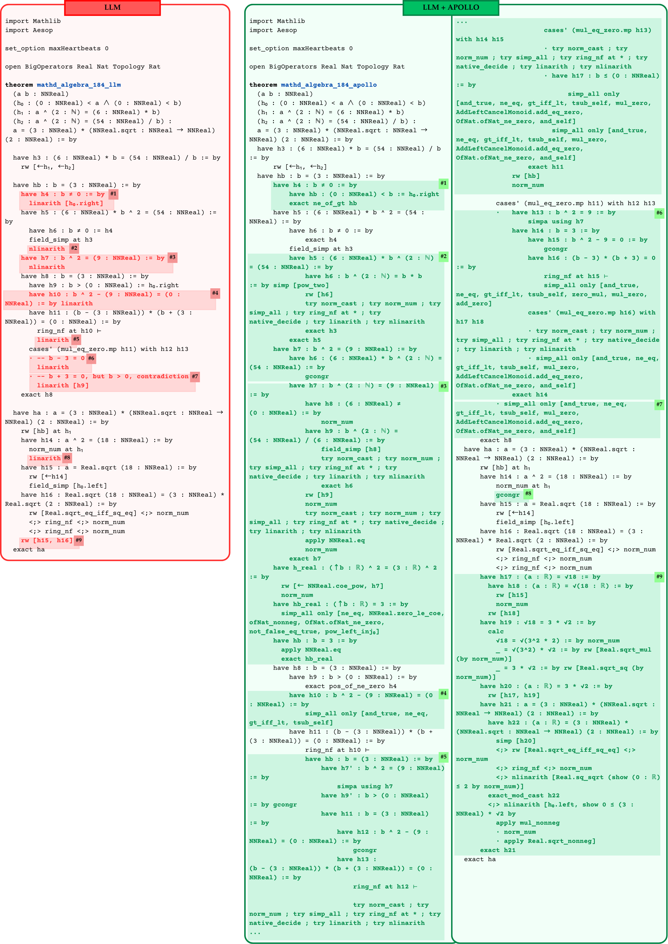
## Code Comparison: LLM vs. LLM + APOLLO ### Overview The image presents a side-by-side comparison of two code implementations, labeled "LLM" (left) and "LLM + APOLLO" (right). Both implementations appear to be attempting to prove the same mathematical theorem, "mathd_algebra_184," within a formal verification environment (likely Lean). The code snippets involve importing libraries, setting options, and defining the theorem with its assumptions and proof steps. The comparison highlights differences in the proof strategies and tactics used in each implementation. ### Components/Axes * **Headers:** * Top-left: "LLM" (enclosed in a red box) * Top-right: "LLM + APOLLO" (enclosed in a green box) * **Code Blocks:** Two distinct blocks of code, one for each implementation. * **Annotations:** Numerical annotations (e.g., "#1", "#2") are scattered throughout both code blocks, potentially indicating key steps or points of divergence. ### Detailed Analysis or ### Content Details Here's a breakdown of the code and annotations, comparing the LLM and LLM + APOLLO implementations: **Common Elements:** * Both implementations start with the same imports: `import Mathlib` and `import Aesop`. * Both set the option `set_option maxHeartbeats 0`. * Both open the namespace `open BigOperators Real Nat Topology Rat`. * Both define the theorem `theorem mathd_algebra_184` with the same assumptions: * `(a b : NNReal)` * `(h₀ : (0 : NNReal) < a ∧ (0 : NNReal) < b)` * `(h₁ : a ^ (2 : ℕ) = (6 : NNReal) * b)` * `(h₂ : a ^ (2 : ℕ) = (54 : NNReal) / b)` * The goal is to prove `a = (3 : NNReal) * (NNReal.sqrt (NNReal → NNReal) (2 : NNReal))` **LLM (Left - Red Box):** * **#1:** `have h4 : b ≠ 0 := by linarith [h₀.right]` * **#2:** `nlinarith` * **#3:** `have h7 : b ^ 2 = (9 : NNReal) := by nlinarith` * **#4:** `have h10 : b ^ 2 - (9 : NNReal) = (0 : NNReal) := by linarith` * **#5:** `linarith` * **#6:** `-- b - 3 = 0` * **#7:** `-- b + 3 = 0, but b > 0, contradiction` * **#8:** `linarith` * **#9:** `rw [h15, h16]` **LLM + APOLLO (Right - Green Box):** * **#1:** `have h4 : b ≠ 0 := by exact ne_of_gt hb` * **#2:** `have h5 : (6 : NNReal) * b ^ (2 : ℕ) = (54 : NNReal) := by have h6 : b ^ (2 : ℕ) = b * b := by simp [pow_two]` * **#3:** `have h7 : b ^ (2 : ℕ) = (9 : NNReal) := by` * **#4:** `have h10 : b ^ 2 - (9 : NNReal) = (0 : NNReal) := by` * **#5:** `have hb : b = (3 : NNReal) := by have h7' : b ^ 2 = (9 : NNReal) simpa using h7` * **#6:** `cases' (mul_eq_zero.mp h16) with` * **#7:** `exact h14` * **#8:** `gcongr` * **#9:** `<;> nlinarith [ho.left, show 0 ≤ (3 : NNReal) * √2 by apply mul_nonneg norm_num apply Real.sqrt_nonneg]` ### Key Observations * The LLM implementation relies heavily on the `nlinarith` tactic, which automatically solves linear arithmetic problems. * The LLM + APOLLO implementation uses more explicit proof steps and tactics, such as `exact ne_of_gt hb`, `simp [pow_two]`, `gcongr`, and `cases'`. * Both implementations arrive at similar intermediate steps, but the level of detail and the tactics used differ significantly. * The annotations highlight specific points where the proof strategies diverge or where particular tactics are applied. ### Interpretation The comparison suggests that the "LLM + APOLLO" implementation provides a more detailed and explicit proof compared to the "LLM" implementation. The LLM implementation leverages the `nlinarith` tactic to automate many of the arithmetic steps, making the proof shorter but potentially less transparent. The "LLM + APOLLO" implementation, on the other hand, breaks down the proof into smaller, more manageable steps, providing greater control and clarity. The choice between the two implementations depends on the desired level of detail and the specific requirements of the verification environment. The annotations serve as valuable markers for understanding the key differences in the proof strategies employed by each implementation.