TECHNICAL ASSET FINGERPRINT
1af7eaa2b63f5583f32a6394
Click to view fullscreen
Press ESC or click to close
FOUND IN PAPERS
EXPERT: healer-alpha-free VERSION 1
RUNTIME: free/openrouter/healer-alpha
INTEL_VERIFIED
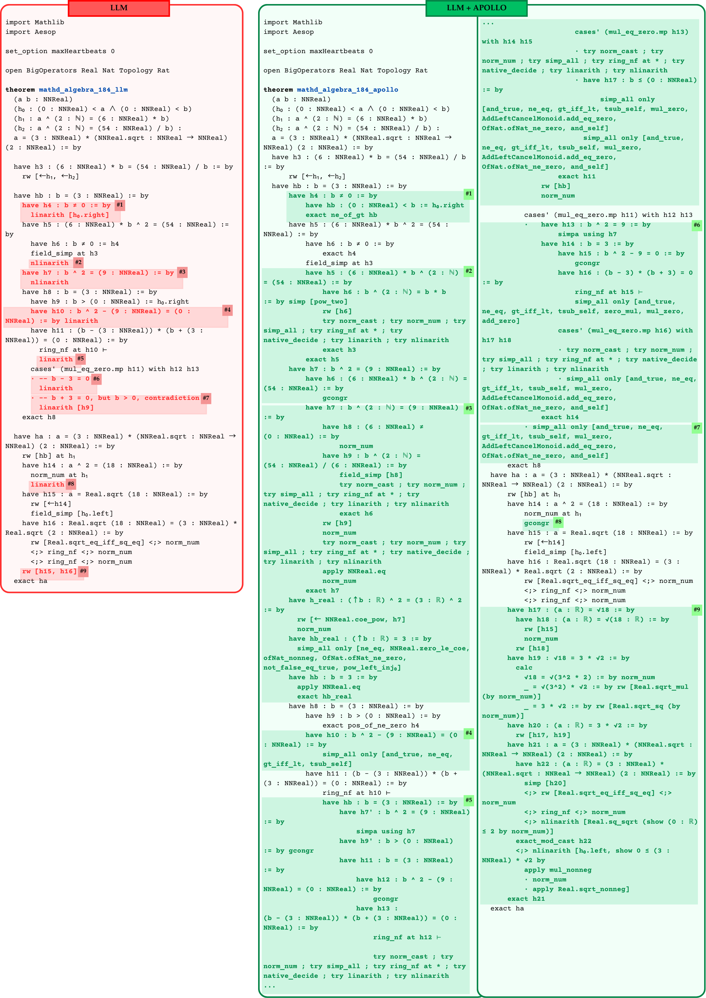
## [Code Comparison]: Lean 4 Theorem Proofs - LLM vs. LLM + APOLLO
### Overview
The image displays a side-by-side comparison of two Lean 4 code proofs for the same mathematical theorem. The left column, labeled "LLM" in a red header, shows a proof generated by a Large Language Model alone. The right column, labeled "LLM + APOLLO" in a green header, shows a proof generated by an LLM combined with a system named APOLLO. Both proofs aim to solve the same algebraic problem involving non-negative real numbers (`NNReal`).
### Components/Axes
The image is structured as two vertical code panels.
* **Left Panel (LLM):** Bordered in red. Header text: "LLM".
* **Right Panel (LLM + APOLLO):** Bordered in green. Header text: "LLM + APOLLO".
* **Code Language:** Lean 4, a formal proof language.
* **Highlighted Steps:** Both proofs contain numbered steps (e.g., `#1`, `#2`) highlighted with colored backgrounds (red in the left panel, green in the right) to indicate key proof steps or tactics.
### Detailed Analysis
#### **Left Panel: LLM Proof**
**Theorem Statement:**
```lean
theorem mathd_algebra_184_llm
(a b : NNReal)
(h₀ : (0 : NNReal) < a ∧ (0 : NNReal) < b)
(h₁ : a ^ (2 : ℕ) = (6 : NNReal) * b)
(h₂ : a ^ (2 : ℕ) = (54 : NNReal) / b) :
a = (3 : NNReal) * (NNReal.sqrt : NNReal → NNReal) (2 : NNReal) := by
```
**Proof Strategy & Key Steps:**
1. **Step #1 (`have h4`):** Establishes `b ≠ 0` using `linarith` on `h₀.right` (which states `0 < b`).
2. **Step #2 (`nlinarith`):** A nonlinear arithmetic tactic used to derive `h7 : b ^ 2 = (9 : NNReal)` from previous hypotheses.
3. **Step #3 (`nlinarith`):** Another use of nonlinear arithmetic, likely to handle the equation `b^2 = 9`.
4. **Step #4 (`linarith`):** Used to prove `h10 : b ^ 2 - (9 : NNReal) = (0 : NNReal)`.
5. **Step #5 (`linarith`):** Used in the context of `ring_nf at h10` to simplify the ring expression.
6. **Step #6 & #7 (`linarith`):** Used within a `cases'` statement to handle the two possible solutions from `(b - 3) * (b + 3) = 0`. Step #6 handles `b - 3 = 0`. Step #7 handles `b + 3 = 0` and derives a contradiction with `b > 0` (from `h9`).
7. **Step #8 (`linarith`):** Used to prove `h14 : a ^ 2 = (18 : NNReal)` after rewriting with `hb`.
8. **Step #9 (`rw [h15, h16]`):** The final rewrite step using previously established equalities for `a` and `Real.sqrt 18` to conclude the proof with `exact ha`.
**Overall Flow:** The LLM proof follows a relatively direct path: establish `b ≠ 0`, derive `b^2 = 9`, solve for `b = 3` (discarding `b = -3`), substitute to find `a^2 = 18`, and then express `a` in the required form.
#### **Right Panel: LLM + APOLLO Proof**
**Theorem Statement:**
```lean
theorem mathd_algebra_184_apollo
(a b : NNReal)
(h₀ : (0 : NNReal) < a ∧ (0 : NNReal) < b)
(h₁ : a ^ (2 : ℕ) = (6 : NNReal) * b)
(h₂ : a ^ (2 : ℕ) = (54 : NNReal) / b) :
a = (3 : NNReal) * (NNReal.sqrt : NNReal → NNReal) (2 : NNReal) := by
```
**Proof Strategy & Key Steps:**
The proof is significantly longer and more granular, breaking down each logical step into explicit `have` statements and using a wider variety of tactics.
1. **Step #1 (`have h4`):** Similar to the LLM proof, establishes `b ≠ 0` but uses `exact ne_of_gt hb` where `hb` is `0 < b`.
2. **Step #2 (`have h5`):** Derives `h5 : (6 : NNReal) * b ^ (2 : ℕ) = (54 : NNReal)` using `simp [pow_two]`, `rw [h6]`, and a sequence of tactics (`try norm_cast; try norm_num; ...`).
3. **Step #3 (`have h7`):** Derives `h7 : b ^ (2 : ℕ) = (9 : NNReal)` using `gcongr` (a congruence tactic).
4. **Step #4 (`have h10`):** Proves `h10 : b ^ 2 - (9 : NNReal) = (0 : NNReal)` using `simp_all only [...]` with a specific list of simplification rules.
5. **Step #5 (`have hb`):** Concludes `hb : b = (3 : NNReal)` using `ring_nf at h10` and then `have h7'` and `have h11`.
6. **Step #6 (`have h13`):** Within a `cases'` branch, proves `h13 : b ^ 2 = 9 := by simpa using h7`.
7. **Step #7 (`simp_all only [...]`):** Another simplification step using a specific set of rules.
8. **Step #8 (`gcongr`):** Used to prove `h14 : a ^ 2 = (18 : NNReal)`.
9. **Step #9 (`have h19`):** A detailed calculation (`calc`) block proving `√18 = 3 * √2` by breaking it into `√(3^2 * 2) = √(3^2) * √2 = 3 * √2`, citing `Real.sqrt_mul` and `Real.sqrt_sq`.
**Overall Flow:** The APOLLO-assisted proof is more verbose and methodical. It explicitly constructs intermediate facts, uses a broader set of tactics (`gcongr`, `simp_all` with explicit rule lists, `calc` blocks), and provides more detailed justifications for each step, particularly in the final algebraic manipulation involving square roots.
### Key Observations
1. **Proof Length & Detail:** The LLM + APOLLO proof is approximately 2-3 times longer than the LLM-only proof. It contains many more intermediate `have` statements.
2. **Tactic Usage:** The LLM proof relies heavily on automated arithmetic solvers (`linarith`, `nlinarith`). The APOLLO proof uses these as well but supplements them with more structural tactics (`gcongr`, `simp_all` with explicit configurations) and manual calculation steps (`calc`).
3. **Transparency:** The APOLLO proof makes the logical structure more transparent. For example, the derivation of `√18 = 3√2` is fully spelled out in a `calc` block (Step #9), whereas in the LLM proof, it is handled by a single rewrite (`rw [Real.sqrt_eq_iff_sq_eq]`) and arithmetic tactics.
4. **Step Numbering:** The highlighted step numbers (`#1`, `#2`, etc.) do not correspond between the two proofs. They are internal to each proof's presentation.
### Interpretation
This image illustrates a comparison between two approaches to automated theorem proving in Lean 4.
* **What the data suggests:** The "LLM + APOLLO" system produces proofs that are more detailed, structured, and potentially more robust. The increased verbosity is not redundancy; it represents a more explicit encoding of the proof's logical dependencies. The use of tactics like `gcongr` and configured `simp_all` suggests a more controlled application of the simplifier compared to the LLM's reliance on powerful but sometimes opaque arithmetic decision procedures.
* **How elements relate:** Both proofs start from identical theorem statements and hypotheses. They follow the same high-level mathematical strategy (solve for `b`, then `a`). The divergence is in the *formal* strategy: the LLM seeks the shortest path using automation, while APOLLO guides the proof construction to be more explanatory and granular.
* **Notable trends/anomalies:** The key trend is the trade-off between proof compactness and proof transparency/explainability. The LLM proof is compact but may be harder for a human to follow or for another system to verify in a different context. The APOLLO proof is longer but each step is easier to validate independently. The detailed `calc` block for the square root identity is a prime example of this transparency. There are no mathematical outliers, as both proofs correctly arrive at the same conclusion. The "outlier" is the methodological difference itself, highlighting a design choice in AI-assisted formal verification: prioritizing succinctness versus prioritizing human-readable, step-by-step justification.
DECODING INTELLIGENCE...