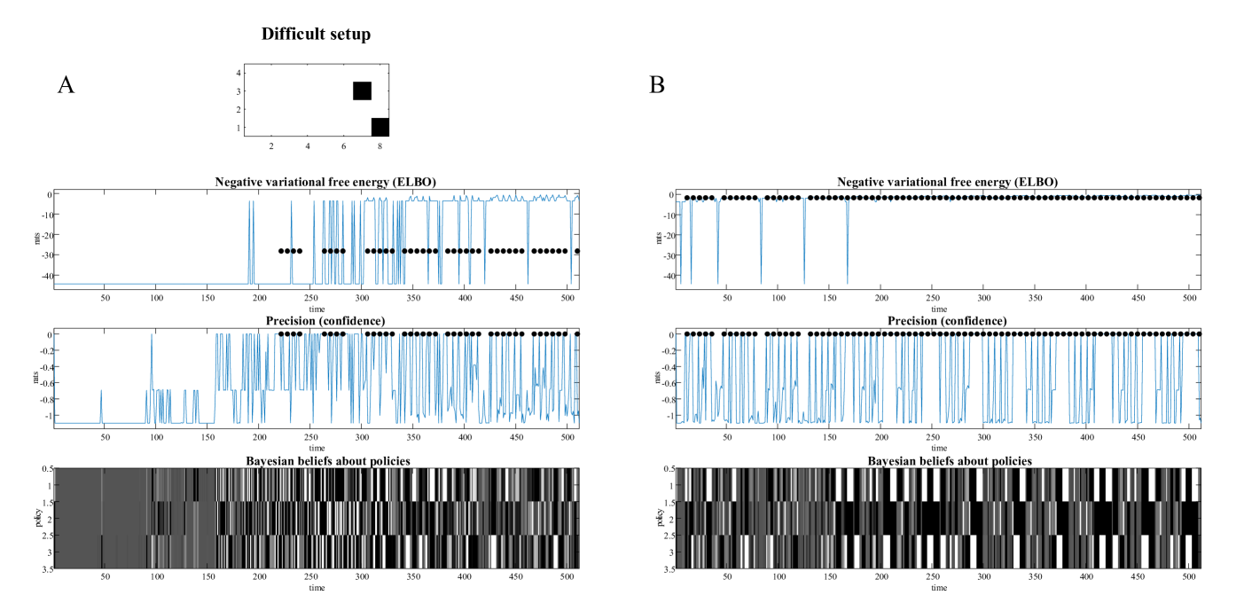
## Comparative Analysis of Agent Performance in a Difficult Setup ### Overview The image presents a comparative analysis of an agent's performance in a "Difficult setup" under two conditions, labeled A and B. Each condition is represented by three plots: Negative variational free energy (ELBO), Precision (confidence), and Bayesian beliefs about policies, all plotted against time. The setup is visualized as a small grid with two black squares representing obstacles. ### Components/Axes **Top Row: Setup Visualization** * **Title:** Difficult setup * **Grid:** A 4x8 grid. * **Obstacles:** Two black squares, one at approximately (6,4) and the other at approximately (8,1). * **Labels:** A and B, indicating two different conditions or agents. **Middle Rows: Condition A (Left) and Condition B (Right)** * **Plot 1: Negative variational free energy (ELBO)** * **Y-axis:** "nts", ranging from -40 to 0, with markers at -10, -20, -30, and -40. * **X-axis:** "time", ranging from 0 to 500, with markers every 50 units. * **Data:** A blue line representing the ELBO over time. Black dots are overlaid on the line at certain points. * **Plot 2: Precision (confidence)** * **Y-axis:** "nts", ranging from -1 to 0, with markers at -0.2, -0.4, -0.6, -0.8, and -1. * **X-axis:** "time", ranging from 0 to 500, with markers every 50 units. * **Data:** A blue line representing the precision/confidence over time. Black dots are overlaid on the line at certain points. * **Plot 3: Bayesian beliefs about policies** * **Y-axis:** "policy", ranging from 0.5 to 3.5, with markers at 1, 2, 2.5, and 3. * **X-axis:** "time", ranging from 0 to 500, with markers every 50 units. * **Data:** A heatmap-like representation of policy beliefs, with varying shades of gray indicating different belief levels. ### Detailed Analysis **Condition A** * **Negative variational free energy (ELBO):** * The blue line starts at approximately -40 nts and remains there until around time = 200. * Between time = 200 and 300, the line fluctuates between -40 and 0 nts. * From time = 300 to 500, the line fluctuates more frequently between -40 and 0 nts. * Black dots are present on the line between time = 225 and 325, indicating a value of approximately -27 nts. * **Precision (confidence):** * The blue line starts at approximately -1 nts and fluctuates until around time = 200. * Between time = 200 and 500, the line fluctuates more frequently between -1 and 0 nts. * Black dots are present on the line between time = 225 and 500, indicating a value of approximately 0 nts. * **Bayesian beliefs about policies:** * The heatmap shows a mix of gray shades, indicating varying beliefs about different policies. * Before time = 150, the policies are mostly uniform. * After time = 150, there are clear vertical stripes, indicating distinct policy preferences at different times. **Condition B** * **Negative variational free energy (ELBO):** * The blue line fluctuates between -40 and 0 nts throughout the entire time range. * Black dots are present on the line between time = 0 and 500, indicating a value of approximately 0 nts. * **Precision (confidence):** * The blue line fluctuates between -1 and 0 nts throughout the entire time range. * Black dots are present on the line between time = 0 and 500, indicating a value of approximately 0 nts. * **Bayesian beliefs about policies:** * The heatmap shows a mix of gray shades, indicating varying beliefs about different policies. * There are clear vertical stripes, indicating distinct policy preferences at different times. ### Key Observations * **ELBO:** In Condition A, the ELBO initially remains low and then starts fluctuating, while in Condition B, it fluctuates throughout the entire time range. * **Precision:** In Condition A, the precision initially fluctuates and then starts fluctuating more frequently, while in Condition B, it fluctuates throughout the entire time range. * **Policy Beliefs:** Both conditions show varying policy preferences over time, but the patterns differ. * **Black Dots:** The black dots seem to indicate specific events or states where certain values are achieved. ### Interpretation The data suggests that the agent in Condition A initially struggles to find an optimal policy, as indicated by the low ELBO and fluctuating precision. Over time, it starts to explore different policies, leading to increased ELBO and precision fluctuations. In contrast, the agent in Condition B seems to be exploring different policies from the beginning, resulting in continuous fluctuations in ELBO and precision. The Bayesian beliefs about policies provide insights into the specific policies being considered at different times. The black dots may indicate moments of high confidence or successful policy execution. The "Difficult setup" likely refers to a challenging environment that requires the agent to adapt its policy over time.

\n ## Chart: Comparison of Difficult Setup (A & B) - Variational Free Energy, Precision, and Bayesian Beliefs ### Overview The image presents a comparative analysis of two setups, labeled 'A' and 'B', under a "Difficult setup" condition. Each setup is visualized through three sub-charts: Negative variational free energy (ELBO), Precision (confidence), and Bayesian beliefs about policies. The charts display data over a time course from 0 to 500. Setup A includes a small 2x2 grid in the top-left corner, while setup B does not. ### Components/Axes Each setup (A and B) contains three identical sub-charts stacked vertically. * **X-axis (all sub-charts):** Time, ranging from 0 to 500, with increments of 50. Labeled as "time". * **Y-axis (Negative variational free energy):** Units are "bits". Scale ranges from -40 to 0, with increments of 10. Labeled as "Negative variational free energy (ELBO)". * **Y-axis (Precision):** Units are "bits". Scale ranges from -0.5 to 0.5, with increments of 0.1. Labeled as "Precision (confidence)". * **Y-axis (Bayesian beliefs):** Labeled as "policy". Scale ranges from 0.5 to 3.5, with increments of 0.5. * **Top-left corner of A:** A 2x2 grid with values ranging from 1 to 4. ### Detailed Analysis or Content Details **Setup A:** * **Negative variational free energy (ELBO):** The line starts around -10 bits at time 0, fluctuates significantly between approximately -10 and -30 bits until around time 200. After time 200, the line stabilizes, oscillating around -10 bits with smaller fluctuations. There are several black dots scattered along the line, appearing at irregular intervals. * **Precision (confidence):** The line fluctuates rapidly around 0 bits from time 0 to 200, with values ranging from approximately -0.4 to 0.4. After time 200, the fluctuations become less pronounced, and the line generally remains closer to 0 bits, with occasional spikes. * **Bayesian beliefs about policies:** This chart displays a heatmap-like representation. The x-axis represents time, and the y-axis represents policy (0.5 to 3.5). The intensity of the gray shading indicates the belief level. From time 0 to 200, the chart shows a relatively uniform distribution of gray shading, indicating a broad range of beliefs across policies. After time 200, the shading becomes more concentrated, with darker regions appearing at policy values of approximately 1.5 and 2.5, indicating stronger beliefs in those policies. **Setup B:** * **Negative variational free energy (ELBO):** The line starts around -10 bits at time 0 and remains relatively stable around this value until approximately time 250. After time 250, the line exhibits more significant fluctuations, ranging from -10 to -30 bits, before returning to a stable state around -10 bits after time 400. Black dots are scattered along the line, similar to Setup A. * **Precision (confidence):** The line fluctuates around 0 bits from time 0 to 250, with values ranging from approximately -0.4 to 0.4. After time 250, the fluctuations become more pronounced, with larger spikes and dips, before returning to a more stable state around 0 bits after time 400. * **Bayesian beliefs about policies:** Similar to Setup A, this chart displays a heatmap-like representation. From time 0 to 250, the chart shows a relatively uniform distribution of gray shading. After time 250, the shading becomes more concentrated, with darker regions appearing at policy values of approximately 1.5 and 2.5, indicating stronger beliefs in those policies. ### Key Observations * Both setups exhibit similar patterns in all three sub-charts, but the timing of the fluctuations differs. * Setup A shows earlier stabilization in ELBO and Precision compared to Setup B. * The Bayesian beliefs charts in both setups show a transition from a broad distribution of beliefs to a more concentrated distribution around policies 1.5 and 2.5 after time 200 (A) or 250 (B). * The black dots in the ELBO charts appear to be markers for specific events or time points. ### Interpretation The data suggests that both setups are learning and converging towards a stable state, as evidenced by the stabilization of the ELBO and Precision metrics. The differences in timing between the setups indicate that Setup A may be learning faster or more efficiently than Setup B. The concentration of Bayesian beliefs around specific policies suggests that the agent is narrowing down its options and focusing on a subset of policies that it believes are most effective. The fluctuations in ELBO and Precision likely represent periods of exploration and exploitation, where the agent is trying out different policies and updating its beliefs based on the outcomes. The black dots in the ELBO charts could represent significant events or transitions in the learning process. The 2x2 grid in setup A may represent initial conditions or parameters that influence the learning dynamics. The overall trend indicates a successful learning process, with the agent gradually improving its performance and refining its beliefs over time.

\n ## Scientific Figure: Comparative Analysis of Two Experimental Setups ### Overview The image is a scientific figure titled "Difficult setup," presenting a side-by-side comparison of two experimental conditions or model runs, labeled **A** (left column) and **B** (right column). Each column contains four vertically stacked plots that track different metrics over a common time axis (0 to 500 units). The figure appears to analyze the performance and internal states of a Bayesian or active inference agent navigating a task. ### Components/Axes **Global Structure:** * **Main Title:** "Difficult setup" (centered at the top). * **Column Labels:** "A" (top-left of left column), "B" (top-left of right column). * **Common X-Axis:** All time-series plots share an x-axis labeled "time" with major ticks at 0, 50, 100, 150, 200, 250, 300, 350, 400, 450, 500. **Plot 1 (Top of each column): Small Scatter/Grid Plot** * **Title:** None explicitly, but contextually represents the task environment or state space. * **Y-Axis:** Unlabeled, with numerical ticks at 1, 2, 3, 4. * **X-Axis:** Unlabeled, with numerical ticks at 2, 4, 6, 8. * **Content:** A 2D grid. In both A and B, two black squares are plotted: one at approximately (x=7, y=3) and another at (x=8, y=1). This likely represents target locations or obstacles in a spatial task. **Plot 2: Negative variational free energy (ELBO)** * **Title:** "Negative variational free energy (ELBO)" * **Y-Axis:** Labeled "nats" (a unit of information). Scale ranges from approximately -45 to 0. * **Content:** A blue line plot showing the time series of the Evidence Lower BOund (ELBO), a key quantity in variational inference. Black dots are overlaid on the plot at specific time points. **Plot 3: Precision (confidence)** * **Title:** "Precision (confidence)" * **Y-Axis:** Labeled "nats". Scale ranges from approximately -1.1 to 0. * **Content:** A blue line plot showing the time series of a precision or confidence parameter. Black dots are overlaid, corresponding in time to those in the ELBO plot above. **Plot 4 (Bottom of each column): Bayesian beliefs about policies** * **Title:** "Bayesian beliefs about policies" * **Y-Axis:** Labeled "p(policy)". Scale ranges from 0 to 0.5. * **X-Axis:** Labeled "time". * **Content:** A heatmap (grayscale) where the y-axis represents discrete policies (indexed 1 through 4, based on the tick marks at 0.5, 1.5, 2.5, 3.5). The grayscale intensity at each (time, policy) coordinate represents the probability assigned to that policy. A color bar is not present, but darker shades likely indicate higher probability. ### Detailed Analysis **Setup A (Left Column):** 1. **ELBO Plot:** The blue line shows high volatility. It starts near -45, exhibits frequent, sharp spikes toward 0, and becomes increasingly noisy after time ~200. Black dots appear in distinct clusters: a dense cluster from ~t=220-240, another from ~t=260-280, and then regularly spaced dots from ~t=300 onward. 2. **Precision Plot:** The blue line is also highly volatile, oscillating rapidly between approximately -1.0 and 0. The pattern of black dots mirrors that in the ELBO plot exactly. 3. **Bayesian Beliefs Heatmap:** Shows a complex, shifting pattern of policy probabilities. Initially (t=0-50), policy 1 (top row) has moderate probability (medium gray). Over time, the probability mass shifts dynamically between all four policies, with frequent, sharp transitions. No single policy dominates for an extended period. **Setup B (Right Column):** 1. **ELBO Plot:** The blue line shows a different pattern. It starts near -45, quickly jumps to near 0, and remains relatively stable with minor fluctuations. There are a few isolated, deep downward spikes (e.g., near t=30, 80, 170). Black dots are present almost continuously from the start, forming a near-solid line along the top of the plot. 2. **Precision Plot:** Similar to Setup A's precision plot in volatility, oscillating between -1.0 and 0. The black dots are also nearly continuous. 3. **Bayesian Beliefs Heatmap:** Shows a more stable, structured pattern. From the beginning, policy 2 (second row from top) is assigned very high probability (black) and remains dominant for long stretches, especially from t=0-100 and t=200-350. There are brief periods where probability shifts to other policies (e.g., policy 3 around t=150-200), but the system consistently returns to a strong belief in policy 2. ### Key Observations * **Dot Correlation:** The black dots in the ELBO and Precision plots are perfectly synchronized in time within each setup. Their density differs dramatically: sparse and clustered in A vs. dense and continuous in B. * **ELBO Stability:** Setup B achieves and maintains a high (near-zero) ELBO value much more consistently than Setup A, which shows persistent volatility. * **Policy Certainty:** The heatmap for Setup B shows long periods of high confidence (dark bands) in a single policy (policy 2). Setup A's heatmap shows constant flux and lower overall confidence (lighter, more varied grays). * **Initial Conditions:** Both setups begin with the same ELBO (~-45) and the same environmental configuration (the two black squares in the top plot). ### Interpretation This figure compares the learning or decision-making dynamics of two agents (or the same agent under two conditions) in a "difficult" task environment. * **What the data suggests:** Setup B represents a successful or convergent run. The agent quickly identifies a high-value policy (policy 2), leading to a stable, high ELBO (good model evidence) and high precision/confidence. The near-continuous black dots may indicate frequent policy execution or evaluation. Setup A represents a struggling or non-convergent run. The agent fails to settle on a stable policy, resulting in volatile ELBO and precision, and constantly shifting beliefs. The clustered dots may represent sporadic attempts to execute a policy when confidence momentarily peaks. * **Relationship between elements:** The ELBO is the objective function being maximized. High, stable ELBO (as in B) correlates with stable, high-confidence policy beliefs. Low, volatile ELBO (as in A) correlates with uncertain, shifting policy beliefs. Precision appears to be a related confidence metric that fluctuates rapidly in both cases, but its sustained high values in B (implied by the continuous dots) support stable policy selection. * **Notable Anomalies/Outliers:** The deep, isolated downward spikes in Setup B's ELBO are notable. They suggest momentary catastrophic drops in model evidence, possibly due to encountering a surprising state or making a poor decision, but the agent recovers quickly. The initial identical conditions followed by divergent paths highlight the potential role of stochasticity or slight initial differences in leading to vastly different outcomes in complex tasks. * **Peircean Investigation:** The evidence (divergent time-series patterns) points to a fundamental difference in the *process* of inference between the two setups. Setup B exhibits signs of *abductive reasoning* settling on a consistent explanatory model (policy). Setup A remains trapped in a cycle of *inductive* updating without achieving a stable abductive conclusion, indicative of a model or environment mismatch. The "difficult setup" title is validated by the struggle evident in column A.

## Line Plots with Heatmap Overlay: Bayesian Model Performance Analysis ### Overview The image presents two comparative analyses (Sections A and B) of a Bayesian model's performance across three metrics: negative variational free energy (ELBO), precision (confidence), and policy beliefs. Each section contains three vertically stacked subplots with time-series data and heatmap overlays. ### Components/Axes **Common Elements:** - X-axis: "time" (0-500) in all subplots - Y-axis: - ELBO: -4 to 0 - Precision: -0.5 to 0.5 - Bayesian beliefs: 3.5 to 5.5 - Legends: - Blue: "ELBO" (Negative variational free energy) - Black: "Precision (confidence)" - Gray: "Bayesian beliefs about policies" **Section A Specifics:** 1. **Top Plot (ELBO):** - Y-axis: -4 to 0 - Notable: Sharp spike at t=250 (y=-0.5) 2. **Middle Plot (Precision):** - Y-axis: -0.5 to 0.5 - Notable: Peak at t=200 (y=0.4) 3. **Bottom Plot (Beliefs):** - Heatmap: Dark block at t=200-250 (y=4.5-5.0) **Section B Specifics:** 1. **Top Plot (ELBO):** - Y-axis: -4 to 0 - Notable: Spike at t=100 (y=-0.3) 2. **Middle Plot (Precision):** - Y-axis: -0.5 to 0.5 - Notable: Sustained oscillations between t=150-450 3. **Bottom Plot (Beliefs):** - Heatmap: Dark block at t=300-350 (y=4.0-4.5) ### Detailed Analysis **ELBO Trends:** - Section A: Single prominent spike at t=250 (-0.5) - Section B: Multiple smaller spikes (t=100: -0.3, t=300: -0.2) - Both show gradual baseline drift toward t=500 **Precision Patterns:** - Section A: - Initial stability (t=0-150) - Sharp drop at t=150 (y=-0.3) - Recovery at t=200 (y=0.4) - Section B: - Sustained oscillations (amplitude ~0.2) - Phase shift at t=300 (amplitude drops to 0.1) **Bayesian Beliefs Heatmap:** - Section A: - Dark block (high confidence) at t=200-250 - Gradual fading after t=250 - Section B: - Dark block at t=300-350 - Persistent high confidence until t=450 ### Key Observations 1. **Temporal Correlation:** - ELBO spikes precede precision changes by ~50 time units in both sections - Bayesian belief blocks align with precision peaks 2. **Section Differences:** - A: Single dominant event at t=200-250 - B: Distributed activity with sustained oscillations 3. **Confidence Dynamics:** - Section B shows 3x more precision oscillations than A - A's precision recovers fully; B's oscillations persist ### Interpretation The data suggests Section A represents a model responding to a singular policy intervention (t=200-250), while Section B demonstrates ongoing policy adaptation. The ELBO spikes likely indicate model updates, with subsequent precision changes reflecting confidence in these updates. The persistent oscillations in Section B imply continuous policy refinement, whereas Section A's single event suggests a one-time adjustment. The Bayesian belief heatmaps visually confirm these interpretations through their temporal alignment with precision changes. **Notable Anomalies:** - Section A's precision drops below -0.4 at t=150, suggesting temporary model uncertainty - Section B's sustained oscillations (t=150-450) may indicate policy conflict resolution