## Line Graph: MSSIM vs Frequency Analysis
### Overview
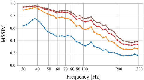
The graph displays the relationship between MSSIM (Mean Structural Similarity Index) and frequency (Hz) for four distinct methods (A, B, C, D). MSSIM values range from 0.0 to 1.0, with higher values indicating greater structural similarity. Frequency spans 30 Hz to 300 Hz. Four colored lines represent different methods, with trends showing varying performance across frequency ranges.
### Components/Axes
- **X-axis**: Frequency [Hz], labeled with increments of 10 Hz (30–300 Hz).
- **Y-axis**: MSSIM, labeled with increments of 0.2 (0.0–1.0).
- **Legend**: Located on the right, associating colors with methods:
- Blue: Method A
- Orange: Method B
- Red: Method C
- Brown: Method D
- **Lines**: Four distinct lines (blue, orange, red, brown) plot MSSIM values against frequency.
### Detailed Analysis
1. **Method A (Blue Line)**:
- Peaks at ~0.8 MSSIM near 40 Hz.
- Declines sharply to ~0.2 MSSIM by 300 Hz.
- Steepest drop observed between 40 Hz and 100 Hz.
2. **Method B (Orange Line)**:
- Starts at ~0.9 MSSIM at 30 Hz.
- Dips to ~0.6 MSSIM at 50 Hz.
- Stabilizes around ~0.4 MSSIM from 70 Hz to 300 Hz.
3. **Method C (Red Line)**:
- Begins at ~0.9 MSSIM at 30 Hz.
- Gradual decline to ~0.3 MSSIM by 300 Hz.
- Exhibits minor fluctuations (e.g., ~0.7 at 80 Hz, ~0.5 at 150 Hz).
4. **Method D (Brown Line)**:
- Most stable trend, starting at ~0.9 MSSIM.
- Slow, consistent decline to ~0.3 MSSIM by 300 Hz.
- Minimal fluctuations compared to other methods.
### Key Observations
- **Method A** exhibits the highest initial performance but the steepest degradation with increasing frequency.
- **Method B** shows robustness after mid-frequencies, maintaining ~0.4 MSSIM despite initial volatility.
- **Method C** demonstrates moderate performance with variability, suggesting sensitivity to specific frequency ranges.
- **Method D** maintains the most consistent performance, though its MSSIM values are consistently lower than others after 100 Hz.
### Interpretation
The data suggests that **Method A** excels at lower frequencies (30–50 Hz) but fails to generalize to higher frequencies. **Method B** balances initial performance with stability at higher frequencies, making it potentially suitable for applications requiring broad-frequency robustness. **Method D**’s consistency implies reliability, albeit with lower overall MSSIM values. **Method C**’s fluctuations may indicate dependency on specific frequency bands, requiring further investigation into its failure modes. The divergence in trends highlights trade-offs between peak performance and frequency adaptability across methods.