## Annotated Aerial Image: Object Detection Results
### Overview
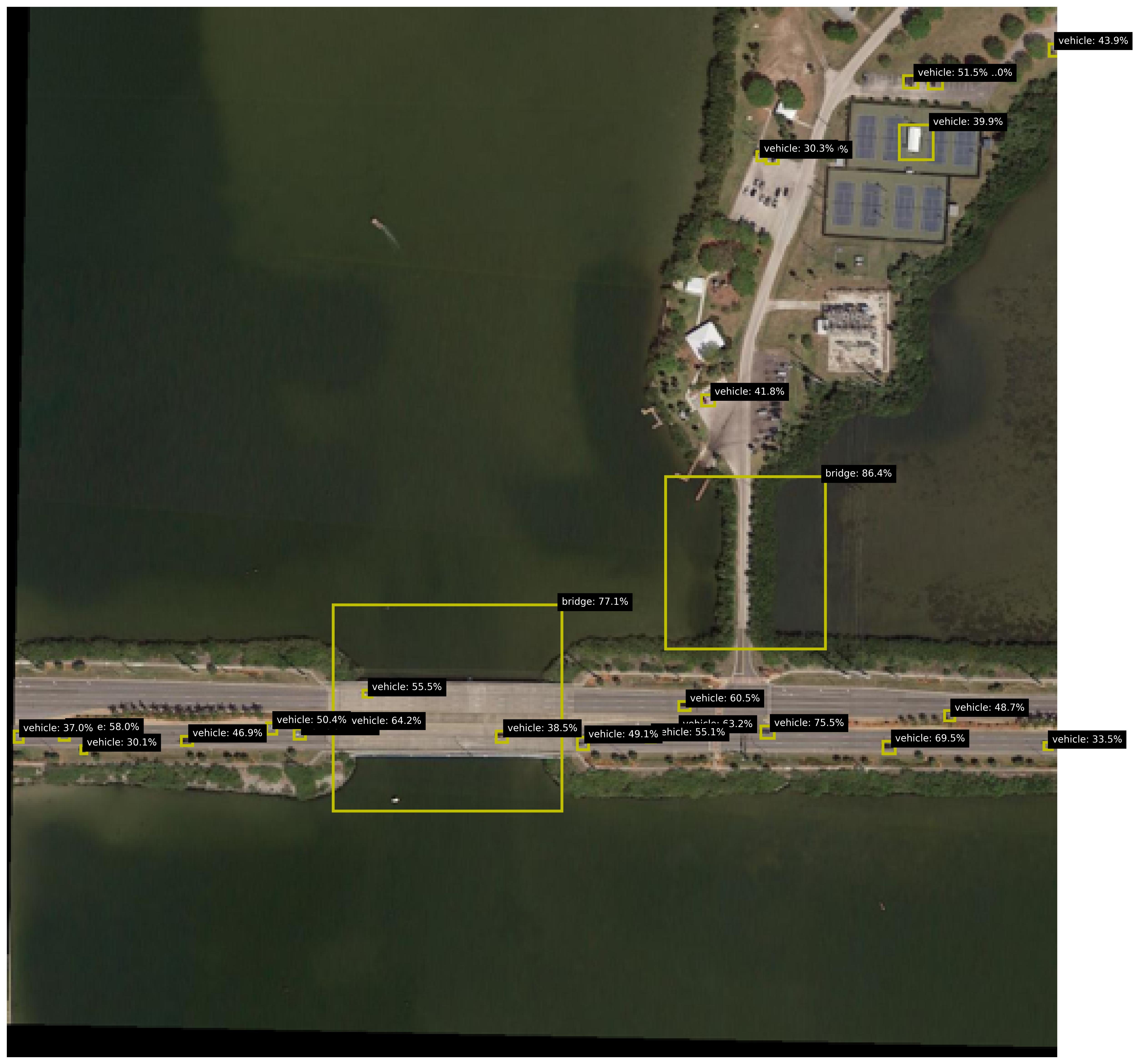
This is a top-down aerial or satellite photograph of a coastal or riverside area, overlaid with the results of an object detection algorithm. The image shows a body of water (dark green/brown), landmasses with vegetation, roads, buildings, and parking areas. Yellow bounding boxes with black text labels have been drawn around detected objects, indicating the object class ("vehicle" or "bridge") and the model's confidence score as a percentage.
### Components/Axes
* **Base Image:** Aerial photograph showing geographical features.
* **Annotations:** Yellow rectangular bounding boxes.
* **Labels:** Black text boxes with white text, positioned at the top-left corner of each bounding box. The format is `[class]: [confidence]%`.
* **Detected Classes:**
* `vehicle`
* `bridge`
* **Spatial Layout:** The image is divided into two primary areas:
1. **Upper Right:** A landmass with buildings, parking lots, and a road leading to a bridge.
2. **Lower Half:** A long, horizontal causeway or bridge structure spanning the water, with a road and vegetation on either side.
### Detailed Analysis
**List of All Detected Objects and Confidence Scores:**
*Upper Right Landmass & Bridge Area (from top to bottom):*
1. `vehicle: 43.9%` (Top-right corner, near edge of frame)
2. `vehicle: 51.5% ..0%` (Note: Label contains "..0%", likely an annotation error or artifact)
3. `vehicle: 39.9%` (On a building roof or parking area)
4. `vehicle: 30.3% %` (Note: Label contains an extra "%" symbol)
5. `vehicle: 41.8%` (On a road near the bridge approach)
6. `bridge: 86.4%` (Large box encompassing the bridge structure connecting to the upper landmass)
*Lower Horizontal Causeway/Bridge (from left to right):*
7. `vehicle: 37.0% e: 58.0%` (Note: Label contains "e: 58.0%", possibly an error or secondary data)
8. `vehicle: 30.1%`
9. `vehicle: 46.9%`
10. `vehicle: 50.4%`
11. `vehicle: 64.2%`
12. `vehicle: 55.5%` (Positioned above the main cluster on the road)
13. `bridge: 77.1%` (Large box encompassing the central section of the causeway over water)
14. `vehicle: 38.5%`
15. `vehicle: 49.1%`
16. `vehicle: 55.1%`
17. `vehicle: 63.2%`
18. `vehicle: 60.5%`
19. `vehicle: 75.5%`
20. `vehicle: 69.5%`
21. `vehicle: 48.7%`
22. `vehicle: 33.5%` (Far right end of the causeway)
### Key Observations
1. **Detection Distribution:** Vehicles are densely clustered along the horizontal causeway/bridge in the lower half of the image, suggesting active traffic flow. A smaller cluster exists in the parking areas on the upper landmass.
2. **Confidence Variability:** Confidence scores for vehicles range widely from ~30% to ~75%. The highest confidence detections (`75.5%`, `69.5%`, `64.2%`) are on the lower causeway. Bridge detections have relatively high confidence (`86.4%`, `77.1%`).
3. **Label Anomalies:** Several labels contain extraneous text (`..0%`, `%`, `e: 58.0%`), which may indicate errors in the annotation overlay process or the presence of additional, non-standard data fields.
4. **Spatial Grounding:** The two `bridge` labels correctly correspond to the two major bridge/causeway structures visible in the image. The `vehicle` labels are all placed on or adjacent to road surfaces and parking areas.
### Interpretation
This image represents the output of a computer vision model performing object detection on aerial imagery. The primary purpose is likely surveillance, traffic monitoring, or infrastructure assessment.
* **What the data suggests:** The model is successfully identifying key infrastructure (bridges) and mobile assets (vehicles). The high confidence on bridges indicates they are distinct, large features the model finds easy to classify. The variable confidence on vehicles may be due to factors like size, occlusion, shadow, or orientation relative to the sensor.
* **How elements relate:** The annotations are directly tied to the visual features in the base photograph. The clustering of vehicle detections on the causeway provides a snapshot of traffic density at the time the image was captured. The two bridges serve as critical choke points or connectors between landmasses.
* **Notable patterns/anomalies:** The most notable pattern is the heavy traffic on the lower causeway versus the lighter activity on the upper landmass roads. The label anomalies (e.g., `e: 58.0%`) are technical artifacts that do not correspond to visible features and should be disregarded as data errors unless their source is understood. The absence of detections on the water (except for a small, unlabelled white object that may be a boat) suggests the model is specifically tuned for land-based objects or that the watercraft did not meet the confidence threshold.