TECHNICAL ASSET FINGERPRINT
1d38db4a870c5cf4b9af06ae
Click to view fullscreen
Press ESC or click to close
FOUND IN PAPERS
EXPERT: healer-alpha-free VERSION 1
RUNTIME: free/openrouter/healer-alpha
INTEL_VERIFIED
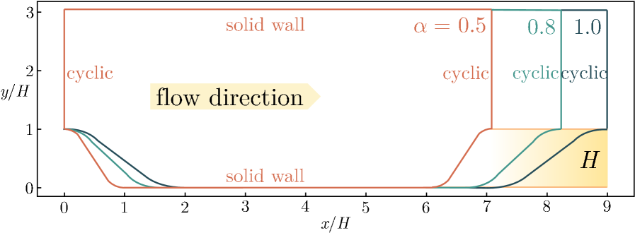
## Diagram: Flow Domain Geometry with Variable Curvature Parameter (α)
### Overview
This image is a technical schematic diagram illustrating a two-dimensional fluid flow domain with three distinct geometric configurations, each defined by a curvature parameter α. The diagram is plotted on a normalized coordinate system (x/H, y/H) and includes boundary condition labels, a flow direction indicator, and a legend for the α values. It appears to be from a computational fluid dynamics (CFD) or fluid mechanics study, showing how a channel's shape varies with α.
### Components/Axes
* **Coordinate System:**
* **X-axis:** Labeled `x/H`, ranging from 0 to 9. This represents the streamwise direction normalized by a characteristic height `H`.
* **Y-axis:** Labeled `y/H`, ranging from 0 to 3. This represents the wall-normal direction normalized by `H`.
* **Boundary Conditions:**
* **Top Boundary (y/H = 3):** Labeled `solid wall` in red text. This is a no-slip or impermeable wall.
* **Bottom Boundary (y/H = 0):** Labeled `solid wall` in red text. This is also a no-slip or impermeable wall.
* **Left Boundary (x/H = 0):** Labeled `cyclic` in red text. This indicates a periodic boundary condition where flow exiting this boundary re-enters from the right.
* **Right Boundary (x/H = 9):** This boundary is segmented into three vertical sections, each labeled `cyclic` in a color matching its corresponding α curve. This indicates that the periodic boundary condition is applied separately for each geometric configuration.
* **Flow Indicator:** A large, light-yellow arrow in the center of the domain points to the right, labeled `flow direction`.
* **Legend / Parameter Key:** Located in the top-right corner of the diagram. It lists three values of the parameter α, each associated with a specific color:
* `α = 0.5` (Red text)
* `0.8` (Teal text)
* `1.0` (Dark green text)
* **Geometric Feature Label:** The shaded area under the right-side curves is labeled with a large, italicized `H` in black, indicating this region represents the characteristic height or a specific geometric feature of size `H`.
### Detailed Analysis
The core of the diagram shows three different channel wall profiles (the lower boundary of the flow domain) that start at (x/H=0, y/H=1) and end at (x/H=9, y/H=1). The upper boundary is a flat, solid wall at y/H=3.
1. **α = 0.5 (Red Curve):**
* **Trend:** The curve exhibits the sharpest curvature. It descends rapidly from y/H=1 at x/H=0, reaches the bottom wall (y/H=0) at approximately x/H=1.5, runs along the bottom wall until about x/H=6.5, then ascends very steeply back to y/H=1 by x/H=7.5.
* **Spatial Grounding:** This creates the narrowest and most abrupt constriction in the channel. The corresponding `cyclic` label on the right boundary is in red and is positioned furthest to the left among the three right-boundary labels.
2. **α = 0.8 (Teal Curve):**
* **Trend:** This curve has a moderate curvature. It descends more gradually than the α=0.5 curve, reaching y/H=0 at approximately x/H=2.5. It runs along the bottom wall until about x/H=7.0, then ascends with a moderate slope, reaching y/H=1 at approximately x/H=8.5.
* **Spatial Grounding:** This creates a channel with a wider and smoother constriction compared to α=0.5. The corresponding `cyclic` label on the right boundary is in teal and is positioned in the middle of the three right-boundary labels.
3. **α = 1.0 (Dark Green Curve):**
* **Trend:** This curve has the gentlest curvature. It descends the most slowly, reaching y/H=0 at approximately x/H=3.5. It runs along the bottom wall until about x/H=7.5, then ascends with the most gradual slope, reaching y/H=1 at approximately x/H=9.0.
* **Spatial Grounding:** This creates the widest and most gradual constriction. The corresponding `cyclic` label on the right boundary is in dark green and is positioned furthest to the right.
The shaded yellow region labeled `H` under the right-side ascent of the curves visually emphasizes the vertical scale of the geometric feature.
### Key Observations
* **Parameter Control:** The parameter α directly controls the "sharpness" or curvature of the channel's lower wall. A lower α (0.5) results in a more abrupt, step-like constriction, while a higher α (1.0) results in a smoother, more gradual ramp.
* **Domain Segmentation:** The right boundary is explicitly divided into three separate cyclic zones, each aligned with the exit of one specific α-geometry. This suggests the diagram may be illustrating three separate computational domains or cases that are being compared.
* **Consistent Start/End Points:** All three geometric profiles share the same inlet (x/H=0, y/H=1) and outlet (x/H=9, y/H=1) vertical positions, isolating the effect of the wall shape between these points.
* **Visual Hierarchy:** The use of color (red, teal, dark green) consistently links the α value in the legend, the corresponding curve, and its associated cyclic boundary label, ensuring clear visual association.
### Interpretation
This diagram is a parametric study of channel geometry. The parameter α likely represents a shape factor in a mathematical function (e.g., a polynomial or trigonometric function) that defines the wall profile. The investigation is probably focused on how this geometric variation affects fluid flow characteristics such as:
* **Pressure Drop:** The sharper constriction (α=0.5) would likely induce a higher pressure loss compared to the smoother one (α=1.0).
* **Flow Separation & Recirculation:** The abrupt change in geometry for α=0.5 is more prone to causing flow separation and recirculation zones (eddies) downstream of the constriction, which could impact mixing or efficiency.
* **Shear Stress Distribution:** The wall shear stress profile along the bottom wall would differ significantly between the three cases due to the varying curvature and local flow acceleration.
The use of cyclic boundaries implies the study is of a periodic flow, such as flow over a repeating array of obstacles or through a corrugated channel, where simulating one full period is sufficient. The diagram serves as a clear, visual definition of the computational or experimental setups being compared, allowing a viewer to immediately grasp the geometric differences between the cases labeled α=0.5, 0.8, and 1.0.
DECODING INTELLIGENCE...