## Line Chart: Throughput vs. Parameter 'm'
### Overview
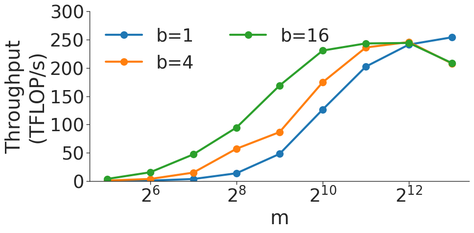
This image displays a line chart illustrating the relationship between a variable 'm' (plotted on a logarithmic x-axis) and system throughput measured in TFLOP/s (y-axis). The chart compares performance across three different configurations of a parameter 'b' (b=1, b=4, b=16). The data demonstrates how increasing the 'b' parameter shifts the performance curve, allowing for higher throughput at smaller values of 'm'.
### Components/Axes
* **Y-Axis:** Labeled "Throughput (TFLOP/s)". The scale is linear, ranging from 0 to 300.
* **X-Axis:** Labeled "m". The scale is logarithmic, with major tick marks at powers of 2 ($2^6, 2^8, 2^{10}, 2^{12}$).
* **Legend:** Positioned in the top-left area.
* **Blue line:** $b=1$
* **Orange line:** $b=4$
* **Green line:** $b=16$
### Detailed Analysis
The chart plots three distinct data series. All series exhibit a sigmoidal (S-curve) growth pattern, where throughput starts near zero, accelerates, and eventually plateaus.
**1. Blue Line ($b=1$):**
* **Trend:** This series shows the slowest growth. It remains near 0 TFLOP/s until $m \approx 2^8$, then begins a steady, steep climb.
* **Data Points (Approximate):**
* $m=2^6$ to $2^8$: $\approx 0-5$ TFLOP/s
* $m=2^9$: $\approx 15$ TFLOP/s
* $m=2^{10}$: $\approx 50$ TFLOP/s
* $m=2^{11}$: $\approx 125$ TFLOP/s
* $m=2^{12}$: $\approx 200$ TFLOP/s
* $m=2^{13}$: $\approx 255$ TFLOP/s (Highest peak of all series)
**2. Orange Line ($b=4$):**
* **Trend:** This series is shifted to the left compared to $b=1$, indicating better performance at lower values of $m$.
* **Data Points (Approximate):**
* $m=2^6$: $\approx 0$ TFLOP/s
* $m=2^7$: $\approx 5$ TFLOP/s
* $m=2^8$: $\approx 15$ TFLOP/s
* $m=2^9$: $\approx 60$ TFLOP/s
* $m=2^{10}$: $\approx 90$ TFLOP/s
* $m=2^{11}$: $\approx 175$ TFLOP/s
* $m=2^{12}$: $\approx 240$ TFLOP/s
**3. Green Line ($b=16$):**
* **Trend:** This series shows the fastest initial growth, reaching high throughput at the lowest $m$ values. However, it exhibits a performance regression (drop) at the highest $m$ value.
* **Data Points (Approximate):**
* $m=2^6$: $\approx 5$ TFLOP/s
* $m=2^7$: $\approx 15$ TFLOP/s
* $m=2^8$: $\approx 50$ TFLOP/s
* $m=2^9$: $\approx 95$ TFLOP/s
* $m=2^{10}$: $\approx 170$ TFLOP/s
* $m=2^{11}$: $\approx 230$ TFLOP/s
* $m=2^{12}$: $\approx 245$ TFLOP/s
* $m=2^{13}$: $\approx 210$ TFLOP/s (Significant drop)
### Key Observations
* **Shift in Saturation:** As the parameter $b$ increases (from 1 to 16), the "knee" of the curve (the point where throughput begins to rise sharply) shifts to the left. This implies that larger $b$ values are more efficient at utilizing hardware resources for smaller problem sizes ($m$).
* **Performance Regression:** The green line ($b=16$) is the only series that shows a clear performance degradation at the largest $m$ value ($2^{13}$), dropping from $\approx 245$ to $\approx 210$ TFLOP/s.
* **Crossover:** The blue line ($b=1$) eventually overtakes the green line at the highest $m$ value, suggesting that while $b=16$ is better for small $m$, $b=1$ is more stable or efficient for very large $m$.
### Interpretation
This chart likely represents a performance benchmark for a computational kernel (such as matrix multiplication or a neural network layer) on a GPU or similar accelerator.
* **Parameter 'm':** Likely represents the matrix dimension or input size.
* **Parameter 'b':** Likely represents the batch size or block size.
* **The "Why":**
* **Small $m$:** Larger batch sizes ($b=16$) are necessary to saturate the compute units. With $b=1$, the workload is too small to keep the hardware busy, resulting in low throughput.
* **Large $m$:** The drop-off in the $b=16$ line at $m=2^{13}$ is a classic indicator of memory bandwidth bottlenecks or cache thrashing. When the batch size is too large combined with a large matrix dimension, the memory footprint likely exceeds the cache capacity, forcing the system to fetch data from slower main memory, thereby reducing throughput.
* **Conclusion:** The optimal configuration depends on the problem size $m$. For smaller $m$, $b=16$ is superior. For very large $m$, $b=1$ is more robust.