## Technical Diagram: Multi-Step Computational Mapping Process
### Overview
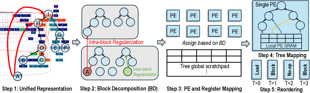
The image is a technical diagram illustrating a five-step process for transforming a complex, interconnected computational graph into an optimized, scheduled execution on a parallel processing architecture. The flow moves from left to right, with each step enclosed in a distinct visual region and labeled sequentially.
### Components/Axes
The diagram is segmented into five primary regions, each representing a step in the pipeline:
1. **Step 1: Unified Representation** (Leftmost region)
2. **Step 2: Block Decomposition (BD)** (Center-left region)
3. **Step 3: PE and Register Mapping** (Center region)
4. **Step 4: Tree Mapping** (Center-right region)
5. **Step 5: Reordering** (Rightmost region)
**Labels and Annotations:**
* **Step Titles:** "Step 1: Unified Representation", "Step 2: Block Decomposition (BD)", "Step 3: PE and Register Mapping", "Step 4: Tree Mapping", "Step 5: Reordering".
* **Process Labels:** "Intra-block Regularization", "Inner-block Regularization", "Assign based on BD".
* **Component Labels:** "PE" (Processing Element), "Tree global scratchpad", "Single PE", "Local PE SRAM".
* **Temporal Labels (Step 5):** "T=0", "T=1", "T=2", "T=3".
* **Node Labels (Step 1):** Letters A through I inside circular nodes.
* **Action Labels (Step 5):** "Load", "Block", "No-op", "Block".
### Detailed Analysis
**Step 1: Unified Representation**
* **Visual:** A complex, non-planar graph with nodes labeled A, B, C, D, E, F, G, H, I. Nodes are connected by a dense network of edges.
* **Spatial Grounding:** Node A is at the bottom-left. Node I is at the top-right. The graph has a layered, somewhat hierarchical appearance but with many cross-connections.
* **Color & Flow:** Red arrows indicate a primary path or dependency chain (e.g., from A to H to I). Blue arrows indicate other connections. The background contains blurred, rectangular elements, possibly representing memory or data blocks.
**Step 2: Block Decomposition (BD)**
* **Visual:** The unified graph is partitioned into two distinct, gray-shaded rectangular blocks.
* **Top Block:** Contains an unlabeled tree structure (root with two children, each with two children).
* **Bottom Block:** Contains a similar tree structure. The leftmost leaf node is highlighted in red and labeled "A". Another node (a right-side leaf) is highlighted in green.
* **Annotations:** A red arrow labeled "Intra-block Regularization" points from the red node (A) to an edge within the top block. A green arrow labeled "Inner-block Regularization" points between two nodes within the bottom block.
**Step 3: PE and Register Mapping**
* **Visual:** Two main components.
1. **Top:** Eight identical light-blue squares arranged in a 2x4 grid, each labeled "PE".
2. **Bottom:** A large rectangle labeled "Tree global scratchpad", subdivided into a grid of 4 columns and at least 3 visible rows (with "..." indicating more).
* **Flow:** The text "Assign based on BD" is positioned between the PE grid and the scratchpad, indicating the mapping logic from the previous decomposition step.
**Step 4: Tree Mapping**
* **Visual:** A detailed view of a "Single PE" (a larger light-blue square). Inside it is a tree structure (similar to those in Step 2) with a yellow arrow tracing a path from a leaf node up to the root.
* **Component:** Below the tree, within the same PE boundary, is a component labeled "Local PE SRAM", depicted as a horizontal row of 8 memory cells.
**Step 5: Reordering**
* **Visual:** Four vertical, light-blue bars representing a schedule or sequence of operations over time.
* **Temporal Sequence:**
* **T=0:** Bar labeled "Load".
* **T=1:** Bar labeled "Block".
* **T=2:** Bar labeled "No-op".
* **T=3:** Bar labeled "Block".
### Key Observations
1. **Progressive Abstraction:** The process moves from a concrete, messy graph (Step 1) to abstract, regularized blocks (Step 2), then to hardware mapping (Steps 3 & 4), and finally to a temporal schedule (Step 5).
2. **Regularization Focus:** Step 2 explicitly introduces "Intra-block" and "Inner-block" regularization, suggesting an optimization pass to structure the decomposed blocks for efficient mapping.
3. **Hierarchy of Memory:** The diagram shows a clear memory hierarchy: a global "Tree global scratchpad" (Step 3) and a per-PE "Local PE SRAM" (Step 4).
4. **Scheduling Insight:** Step 5 reveals that the final execution is not a simple linear flow. The "No-op" at T=2 indicates a pipeline bubble or deliberate stall, and the repeated "Block" operation suggests a chunk-based or batched processing model.
### Interpretation
This diagram outlines a compiler or runtime system's methodology for mapping an arbitrary computational graph (e.g., a neural network layer, a dataflow program) onto a parallel hardware accelerator composed of multiple Processing Elements (PEs) with local memory.
The **core investigative reading** is as follows:
1. **Problem:** The initial graph (Step 1) is irregular and not directly mappable to hardware.
2. **Solution - Decomposition & Regularization (Step 2):** The graph is broken into subgraphs (blocks). Regularization techniques are applied to simplify connections within and between these blocks, making them more amenable to parallel execution. The highlighting of node 'A' suggests it may be a critical or anchor node in this process.
3. **Solution - Hardware Mapping (Steps 3 & 4):** The regularized blocks are assigned to physical PEs. The "Tree global scratchpad" likely holds intermediate data shared between PEs. Step 4 shows how a single block's tree structure is mapped into a PE's local memory and execution unit, with the yellow arrow possibly representing a specific computation path or reduction operation.
4. **Solution - Temporal Orchestration (Step 5):** The final step schedules the operations. The sequence "Load -> Block -> No-op -> Block" implies a phased execution: first loading data/weights, then processing a block of work, followed by a synchronization point or memory operation (the No-op), and then processing another block. This pattern is typical in systolic arrays or wavefront architectures to manage data dependencies and pipeline efficiency.
**Notable Anomaly:** The "No-op" cycle is significant. It is not idle time but a necessary part of the schedule, likely for waiting on data from another PE, flushing a pipeline, or aligning with a global synchronization barrier. This highlights that optimal mapping requires careful temporal planning, not just spatial assignment.
**Conclusion:** The diagram is a high-level schematic for a graph-to-hardware compilation pipeline, emphasizing decomposition, regularization, spatial mapping to a PE array, and the creation of a synchronized, multi-cycle execution schedule.