## Diagram: Array Contribution Computation Process
### Overview
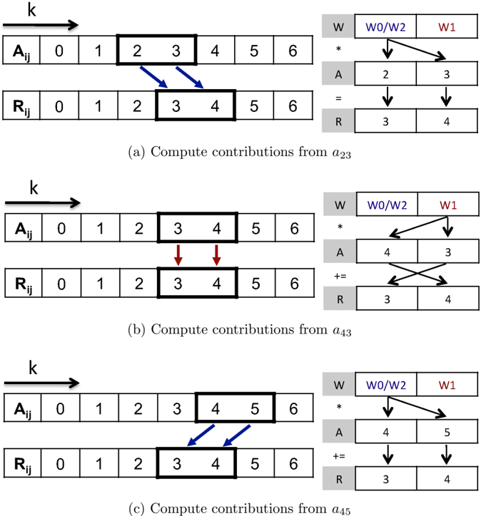
The image displays three distinct panels, labeled (a), (b), and (c), illustrating a computational process involving two arrays, $A_{ij}$ (input) and $R_{ij}$ (result/output). The diagrams demonstrate how specific elements from the input array are selected, processed via weights, and contributed to the result array. This is characteristic of a sliding window operation, such as a 1D convolution or stencil computation.
### Components/Axes
* **Arrays ($A_{ij}$ and $R_{ij}$):** Horizontal arrays with indices labeled 0 through 6.
* **Selection Boxes:** Bold black rectangles highlighting two adjacent indices in the arrays.
* **Operation Tables (Right-hand side):**
* **W:** Represents weights, labeled "W0/W2" (blue text) and "W1" (red text).
* **\***: Multiplication operation.
* **A:** Input values selected from the array.
* **= / +=:** Assignment or accumulation operation.
* **R:** Resulting values in the output array.
* **Arrows:**
* **Blue Arrows:** Indicate direct mapping/contribution.
* **Red Arrows:** Indicate direct mapping/contribution (specifically in panel b).
* **Black Arrows:** Indicate flow within the operation tables.
---
### Detailed Analysis
#### Panel (a): Compute contributions from $a_{23}$
* **Array State:** The box in $A_{ij}$ highlights indices 2 and 3 (values 2 and 3). The box in $R_{ij}$ highlights indices 3 and 4 (values 3 and 4).
* **Flow:** Blue arrows connect $A_{ij}$ indices 2 and 3 to $R_{ij}$ indices 3 and 4.
* **Operation Table:**
* Weights: W0/W2 (blue) and W1 (red).
* Input A: 2 and 3.
* Result R: 3 and 4.
* The table shows the multiplication of weights with input values and assignment to the result.
#### Panel (b): Compute contributions from $a_{43}$
* **Array State:** The box in $A_{ij}$ highlights indices 3 and 4 (values 3 and 4). The box in $R_{ij}$ highlights indices 3 and 4 (values 3 and 4).
* **Flow:** Red arrows connect $A_{ij}$ indices 3 and 4 to $R_{ij}$ indices 3 and 4.
* **Operation Table:**
* Weights: W0/W2 (blue) and W1 (red).
* Input A: 4 and 3.
* Result R: 3 and 4.
* **Note:** The table shows a cross-over pattern where the input value 4 (from index 3) and 3 (from index 4) are mapped to result indices 3 and 4 respectively using the "+=" (accumulation) operator.
#### Panel (c): Compute contributions from $a_{45}$
* **Array State:** The box in $A_{ij}$ highlights indices 4 and 5 (values 4 and 5). The box in $R_{ij}$ highlights indices 3 and 4 (values 3 and 4).
* **Flow:** Blue arrows connect $A_{ij}$ indices 4 and 5 to $R_{ij}$ indices 3 and 4.
* **Operation Table:**
* Weights: W0/W2 (blue) and W1 (red).
* Input A: 4 and 5.
* Result R: 3 and 4.
* The table shows the multiplication of weights with input values and accumulation into the result.
---
### Key Observations
* **Sliding Window:** The input array $A_{ij}$ window moves from indices [2,3] to [3,4] to [4,5].
* **Fixed Output:** The output array $R_{ij}$ window remains fixed at indices [3,4] across all three panels.
* **Accumulation Logic:** Panels (b) and (c) use the "+=" operator, implying that the result array $R_{ij}$ is being built up incrementally by summing contributions from different windows of the input array.
* **Weight Application:** The weights "W0/W2" and "W1" are applied consistently across all operations, suggesting a filter kernel of size 2.
### Interpretation
This diagram illustrates the mechanics of a **1D Convolution** or a **Stencil Computation**.
* **The Process:** The system is sliding a kernel (represented by the weights W0/W2 and W1) across an input array $A$. As the kernel slides, it performs a weighted sum (or similar operation) and accumulates the result into a specific region of the output array $R$.
* **Why it matters:** This is a fundamental operation in signal processing, image processing (e.g., blurring, edge detection), and deep learning (convolutional neural networks). The diagram explicitly shows how a single output element (or range of elements) is influenced by multiple input elements over time/iterations.
* **The "Why":** The use of "+=" in panels (b) and (c) indicates that the output array is not just a direct mapping, but an accumulation buffer. This is typical in parallel computing or hardware acceleration (like FPGAs or GPUs) where partial sums are computed and added to a global result array. The "cross-over" in panel (b) suggests a specific data permutation or reordering step often required to align data for efficient parallel processing.