## Technical Diagram: Computation of Contributions in a Weighted Array Operation ### Overview The image is a technical diagram illustrating a three-step computational process for calculating contributions from specific elements of a source array (`A_ij`) to a result array (`R_ij`), using a set of weights (`W`). The diagram is divided into three horizontally stacked panels, labeled (a), (b), and (c), each depicting a distinct step in the sequence. The overall process appears to be a form of weighted accumulation or convolution, common in signal processing or neural network computations. ### Components/Axes The diagram does not have traditional chart axes. Its components are: * **Primary Arrays (Left Side):** Two horizontal arrays are shown in each panel. * `A_ij`: The source array, indexed from 0 to 6. A specific contiguous block of two elements is highlighted with a bold black outline in each step. * `R_ij`: The result array, also indexed from 0 to 6. A specific contiguous block of two elements (indices 3 and 4) is highlighted with a bold black outline in each step. * **Computation Diagram (Right Side):** A smaller schematic for each panel shows the detailed operation. * `W`: A weight vector with two elements. The first element is labeled `W0/W2` (in blue text), and the second is `W1` (in red text). * `A`: A vector containing the two values selected from the `A_ij` array for that step. * `R`: The corresponding two values from the `R_ij` array being updated. * **Arrows & Operators:** Arrows indicate data flow. The operator between the `W` and `A` vectors is `*` (multiplication). The operator leading to the `R` vector is either `=` (assignment) or `+=` (addition/accumulation). * **Directional Indicator:** An arrow labeled `k` points to the right above each `A_ij` array, indicating the direction of index progression. 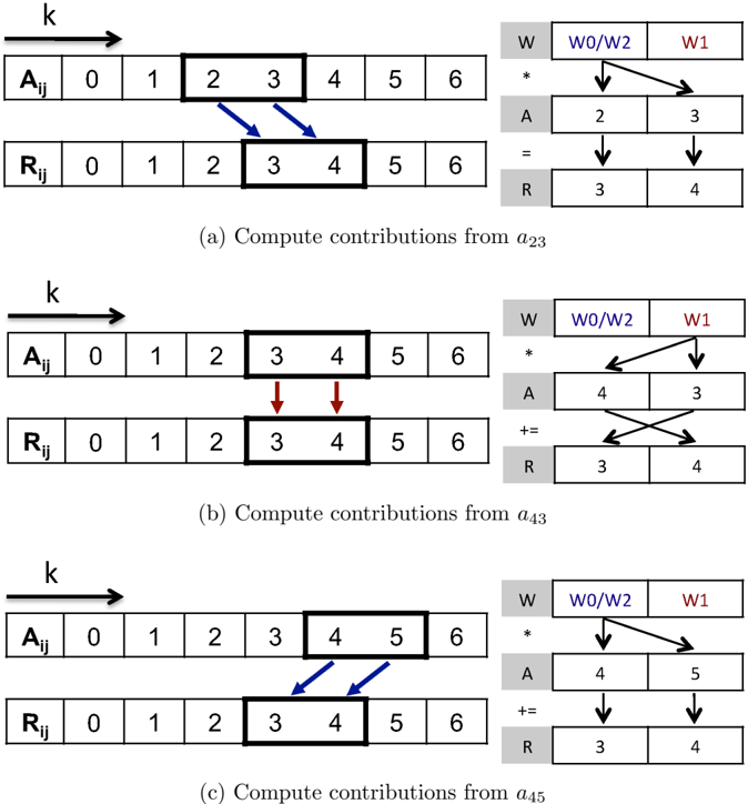* **Panel Labels:** Each panel has a caption: * (a) Compute contributions from `a_23` * (b) Compute contributions from `a_43` * (c) Compute contributions from `a_45` ### Detailed Analysis The process is broken down into three sequential steps, each computing the contribution from a different element of `A_ij` to the result array `R_ij[3]` and `R_ij[4]`. **Panel (a): Compute contributions from `a_23`** * **Source Selection:** The elements `A_ij[2]` and `A_ij[3]` (with values 2 and 3, respectively) are selected. * **Computation Flow:** 1. The weight `W0/W2` (blue) is multiplied by `A[2]` (value 2). 2. The weight `W1` (red) is multiplied by `A[3]` (value 3). 3. The results are assigned (`=`) to `R[3]` and `R[4]`, setting them to 3 and 4. * **Visual Cues:** Blue arrows connect the selected `A_ij` elements to the computation. The operation is an initial assignment. **Panel (b): Compute contributions from `a_43`** * **Source Selection:** The elements `A_ij[3]` and `A_ij[4]` (with values 3 and 4, respectively) are selected. * **Computation Flow:** 1. The weight `W0/W2` (blue) is multiplied by `A[4]` (value 4). 2. The weight `W1` (red) is multiplied by `A[3]` (value 3). 3. The results are accumulated (`+=`) into the existing `R[3]` and `R[4]`. The diagram shows a cross-connection: the product of `W0/W2 * A[4]` is added to `R[4]`, and the product of `W1 * A[3]` is added to `R[3]`. * **Visual Cues:** Red arrows connect the selected `A_ij` elements. The operation is an accumulation. **Panel (c): Compute contributions from `a_45`** * **Source Selection:** The elements `A_ij[4]` and `A_ij[5]` (with values 4 and 5, respectively) are selected. * **Computation Flow:** 1. The weight `W0/W2` (blue) is multiplied by `A[4]` (value 4). 2. The weight `W1` (red) is multiplied by `A[5]` (value 5). 3. The results are accumulated (`+=`) into `R[3]` and `R[4]`. The arrows show a direct mapping: `W0/W2 * A[4]` is added to `R[3]`, and `W1 * A[5]` is added to `R[4]`. * **Visual Cues:** Blue arrows connect the selected `A_ij` elements. The operation is an accumulation. ### Key Observations 1. **Sliding Window:** The computation uses a sliding window of size 2 over the `A_ij` array. The window moves from indices [2,3] to [3,4] to [4,5]. 2. **Fixed Output Window:** Despite the moving input window, the output is always written to the fixed window `R_ij[3]` and `R_ij[4]`. 3. **Weight Reuse & Mapping:** The same two weights (`W0/W2` and `W1`) are reused in each step. The mapping from the product `(weight * A_value)` to the output index `R[3]` or `R[4]` changes between steps, particularly in the cross-connection seen in panel (b). 4. **Operation Sequence:** The first step (a) is an assignment (`=`), initializing the values in `R[3]` and `R[4]`. Subsequent steps (b and c) are accumulations (`+=`), adding to those initial values. 5. **Color Coding:** Blue is consistently associated with `W0/W2` and the first element of the selected `A` pair. Red is associated with `W1` and the second element of the selected `A` pair. The arrow colors (blue in a/c, red in b) may highlight which step is being emphasized or the primary data flow for that step. ### Interpretation This diagram illustrates a specific algorithm for computing a localized, weighted sum. It demonstrates how contributions from different parts of an input array (`A_ij`) are aggregated into a fixed region of an output array (`R_ij`). * **What it suggests:** The process is likely a visualization of a **convolution** or a **sliding window dot product** operation, where a kernel (the weights `W`) is applied across an input signal (`A_ij`). However, the fixed output window and the specific cross-mapping in step (b) suggest a more specialized operation, possibly related to **attention mechanisms**, **sparse updates**, or a **specific hardware/dataflow optimization** where data from different input positions is routed to the same output location. * **Relationships:** The core relationship is between the moving input window, the static weight vector, and the fixed output window. The diagram emphasizes the data dependency and routing logic—*which* input element, multiplied by *which* weight, contributes to *which* output element at each step. * **Notable Anomalies:** The cross-connection in panel (b) is the most notable feature. It breaks the simple left-to-right mapping seen in (a) and (c). This implies the algorithm is not a straightforward convolution but has a specific, non-linear indexing or routing rule. The label `W0/W2` also hints that this weight might be shared or have dual roles in a larger system not fully depicted here. **Language Note:** All text in the diagram is in English. Mathematical notation (subscripts like `ij`, `a_23`) is used.