\n
## Violin Plot Comparison: FairPFN vs. Unfair Methods for Predicted Causal Effect (ATE) Under Varying Noise Levels
### Overview
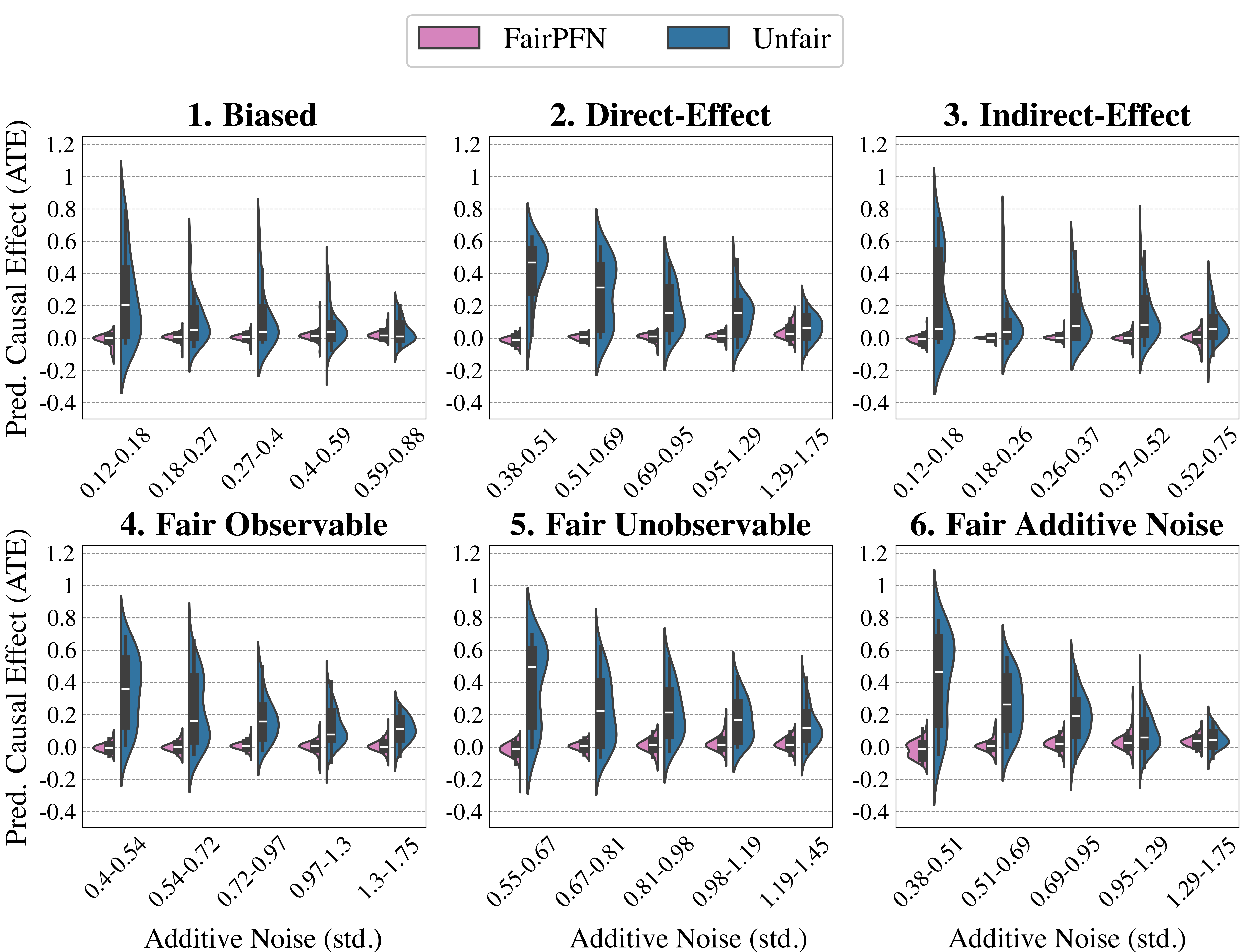
The image displays a 2x3 grid of six violin plots. Each plot compares the distribution of Predicted Average Treatment Effect (ATE) for two methods, "FairPFN" (pink) and "Unfair" (blue), across five increasing levels of additive noise (standard deviation). The plots are organized by different causal scenarios or data-generating processes.
### Components/Axes
* **Legend:** Located at the top center of the entire figure.
* Pink rectangle: **FairPFN**
* Blue rectangle: **Unfair**
* **Y-Axis (Common to all plots):** Label: **Pred. Causal Effect (ATE)**. Scale ranges from -0.4 to 1.2, with major gridlines at intervals of 0.2.
* **X-Axis (Common label):** Label: **Additive Noise (std.)**. The specific numeric ranges for the five bins vary per subplot.
* **Subplot Titles (2 rows, 3 columns):**
1. **1. Biased** (Top Left)
2. **2. Direct-Effect** (Top Center)
3. **3. Indirect-Effect** (Top Right)
4. **4. Fair Observable** (Bottom Left)
5. **5. Fair Unobservable** (Bottom Center)
6. **6. Fair Additive Noise** (Bottom Right)
### Detailed Analysis
Each subplot contains five pairs of violin plots (one pink, one blue per noise bin). The violin shows the probability density of the data, with a white dot marking the median, a thick black bar for the interquartile range, and thin black lines for the whiskers.
**1. Biased**
* **X-axis Bins:** 0.12-0.18, 0.18-0.27, 0.27-0.4, 0.4-0.59, 0.59-0.88
* **Trend:** The "Unfair" (blue) distributions are wide, with medians starting high (~0.2) and decreasing as noise increases. The "FairPFN" (pink) distributions are extremely tight and centered near zero across all noise levels.
**2. Direct-Effect**
* **X-axis Bins:** 0.38-0.51, 0.51-0.69, 0.69-0.95, 0.95-1.29, 1.29-1.75
* **Trend:** Similar to plot 1. "Unfair" medians start high (~0.5) and decline. "FairPFN" remains tightly clustered around zero.
**3. Indirect-Effect**
* **X-axis Bins:** 0.12-0.18, 0.18-0.26, 0.26-0.37, 0.37-0.52, 0.52-0.75
* **Trend:** "Unfair" distributions are tall and narrow, with medians starting very high (~0.6) and decreasing. "FairPFN" is again tightly centered near zero.
**4. Fair Observable**
* **X-axis Bins:** 0.4-0.54, 0.54-0.72, 0.72-0.97, 0.97-1.3, 1.3-1.75
* **Trend:** "Unfair" medians start moderately high (~0.4) and decrease. "FairPFN" distributions are slightly wider than in previous plots but still tightly centered near zero.
**5. Fair Unobservable**
* **X-axis Bins:** 0.55-0.67, 0.67-0.81, 0.81-0.98, 0.98-1.19, 1.19-1.45
* **Trend:** "Unfair" distributions are wide, with medians starting high (~0.5) and decreasing. "FairPFN" is tightly centered near zero.
**6. Fair Additive Noise**
* **X-axis Bins:** 0.38-0.51, 0.51-0.69, 0.69-0.95, 0.95-1.29, 1.29-1.75
* **Trend:** "Unfair" medians start high (~0.5) and decrease. "FairPFN" is tightly centered near zero.
### Key Observations
1. **Consistent FairPFN Performance:** Across all six causal scenarios and all noise levels, the "FairPFN" method produces predicted ATE distributions that are consistently narrow and centered very close to zero (the ideal for a fair estimator).
2. **Unfair Method Bias:** The "Unfair" method shows significant positive bias (median ATE > 0) in all scenarios, especially at lower noise levels. This bias decreases as additive noise increases.
3. **Noise Impact:** Increasing additive noise (moving right on the x-axis within each plot) generally reduces the variance and median of the "Unfair" method's predictions, pulling them closer to zero, but they rarely achieve the tight, zero-centered precision of "FairPFN".
4. **Scenario Sensitivity:** The "Unfair" method's starting bias and the shape of its distribution vary across the six causal scenarios (e.g., highest initial median in "Indirect-Effect"), while "FairPFN" is robust to these differences.
### Interpretation
This figure demonstrates the effectiveness of the "FairPFN" method in estimating causal effects fairly (i.e., with near-zero bias) compared to an "Unfair" baseline, under varying conditions of data corruption (additive noise) and different underlying causal structures.
* **What the data suggests:** The "FairPFN" method successfully mitigates bias in predicted Average Treatment Effects. Its tight distributions around zero indicate high precision and fairness. The "Unfair" method is susceptible to significant bias, which is only reduced by increasing noise—a factor that also degrades the signal.
* **Relationship between elements:** The six panels show that the advantage of FairPFN is not scenario-specific; it holds across a taxonomy of causal problems (Biased, Direct/Indirect Effect, and various Fairness definitions). The x-axis (noise) acts as a stress test, showing FairPFN's robustness.
* **Notable patterns/anomalies:** The most striking pattern is the stark contrast in distribution shape and location between the two methods in every single bin. There are no outliers where the "Unfair" method outperforms "FairPFN" in terms of fairness (closeness to zero). The "Indirect-Effect" scenario appears to induce the strongest bias in the "Unfair" method at low noise levels.