## Code Comparison: LLM vs. LLM + APOLLO
### Overview
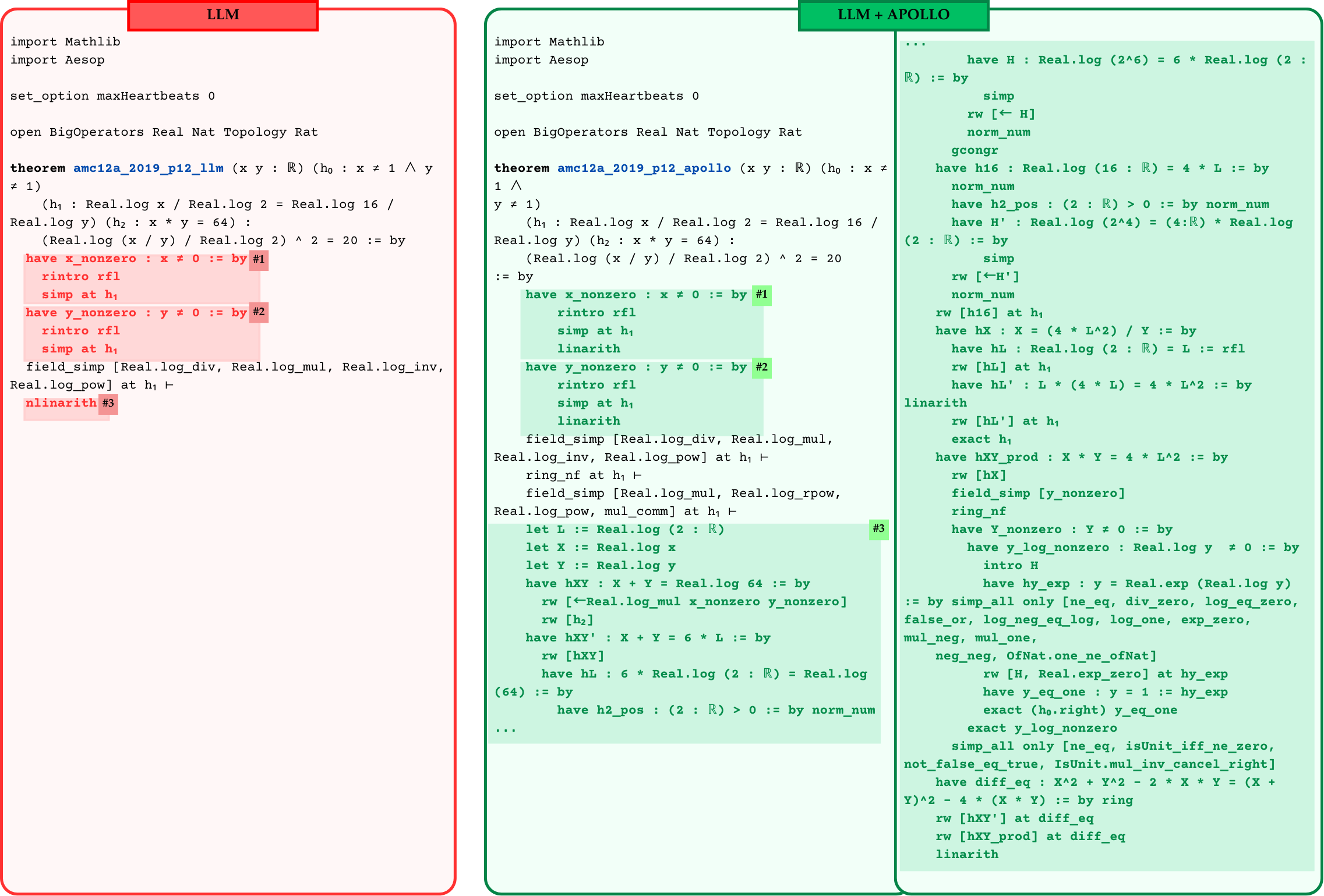
The image presents a side-by-side comparison of code snippets, labeled "LLM" (left) and "LLM + APOLLO" (right), likely representing different approaches or versions of a mathematical proof or computation. The code appears to be written in a language related to theorem proving or formal verification, possibly Lean. The comparison highlights differences in the code structure and specific commands used.
### Components/Axes
* **Headers:**
* Left: "LLM" (red background)
* Right: "LLM + APOLLO" (green background)
* **Code Blocks:** Two distinct code blocks, one under each header.
* **Annotations:** Numerical annotations (#1, #2, #3) highlight specific lines or sections in each code block.
* The code includes imports, options settings, theorem definitions, and proof steps.
### Detailed Analysis or ### Content Details
**Left Code Block (LLM):**
```lean
import Mathlib
import Aesop
set_option maxHeartbeats 0
open BigOperators Real Nat Topology Rat
theorem amc12a_2019_p12_1lm (x y : R) (h₀ : x ≠ 1 ∧ y ≠ 1)
(h₁ : Real.log x / Real.log 2 = Real.log 16 / Real.log y) (h₂ : x * y = 64) :
(Real.log (x / y) / Real.log 2) ^ 2 = 20 := by
have x_nonzero : x ≠ 0 := by #1
rintro rfl
simp at h₁
have y_nonzero : y ≠ 0 := by #2
rintro rfl
simp at h₁
field_simp [Real.log_div, Real.log_mul, Real.log_inv, Real.log_pow] at h₁
nlinarith #3
```
**Right Code Block (LLM + APOLLO):**
```lean
import Mathlib
import Aesop
set_option maxHeartbeats 0
open BigOperators Real Nat Topology Rat
theorem amc12a_2019_p12_apollo (x y : R) (h₀ : x ≠ 1 ∧ y ≠ 1)
(h₁ : Real.log x / Real.log 2 = Real.log 16 / Real.log y) (h₂ : x * y = 64) :
(Real.log (x / y) / Real.log 2) ^ 2 = 20 := by
have x_nonzero : x ≠ 0 := by #1
rintro rfl
simp at h₁
linarith
have y_nonzero : y ≠ 0 := by #2
rintro rfl
simp at h₁
linarith
field_simp [Real.log_div, Real.log_mul, Real.log_inv, Real.log_pow] at h₁
ring_nf at h₁
field_simp [Real.log_mul, Real.log_rpow, Real.log_pow, mul_comm] at h₁
let L := Real.log (2 : R)
let X := Real.log x
let Y := Real.log y
have hXY : X + Y = Real.log 64 := by
rw [Real.log_mul x_nonzero y_nonzero]
rw [h₂]
have hXY' : X + Y = 6 * L := by
rw [hXY]
have hL : 6 * Real.log (2 : R) = Real.log (64) := by
have h₂_pos : (2 : R) > 0 := by norm_num
have H : Real.log (2^6) = 6 * Real.log (2 : R) := by
simp
rw [← H]
norm_num
gcongr
have h16 : Real.log (16 : R) = 4 * L := by
norm_num
have h₂_pos : (2 : R) > 0 := by norm_num
have H' : Real.log (2^4) = (4 : R) * Real.log (2 : R) := by
simp
rw [← H']
norm_num
rw [h16] at h₁
have hX : X = (4 * L^2) / Y := by
have hL : Real.log (2 : R) = L := rfl
rw [hL] at h₁
have hL' : L * (4 * L) = 4 * L^2 := by
linarith
rw [hL'] at h₁
exact h₁
have hXY_prod : X * Y = 4 * L^2 := by
rw [hX]
field_simp [y_nonzero]
ring_nf
have Y_nonzero : Y ≠ 0 := by
have y_log_nonzero : Real.log y ≠ 0 := by
intro H
have hy_exp : y = Real.exp (Real.log y) := by simp_all only [ne_eq, div_zero, log_eq_zero, false_or, log_neg_eq_log, log_one, exp_zero, mul_neg, mul_one, neg_neg, OfNat.one_ne_ofNat]
rw [H, Real.exp_zero] at hy_exp
have y_eq_one : y = 1 := hy_exp
exact (h₀.right) y_eq_one
exact y_log_nonzero
simp_all only [ne_eq, isUnit_iff_ne_zero, not_false_eq_true, IsUnit.mul_inv_cancel_right]
have diff_eq : X^2 + Y^2 - 2 * X * Y = (X + Y)^2 - 4 * (X * Y) := by ring
rw [hXY'] at diff_eq
rw [hXY_prod] at diff_eq
linarith
```
**Annotations:**
* `#1`: Marks the "have x_nonzero" line in both code blocks.
* `#2`: Marks the "have y_nonzero" line in both code blocks.
* `#3`: Marks the "nlinarith" line in the LLM code block and a section of code starting with `let L := Real.log (2 : R)` in the LLM + APOLLO code block.
### Key Observations
* The "LLM + APOLLO" code block is significantly longer and more detailed than the "LLM" code block.
* The "LLM" code uses `nlinarith` to complete the proof, while "LLM + APOLLO" expands the proof with more explicit steps.
* The "LLM + APOLLO" code introduces intermediate variables (L, X, Y) and uses rewrite rules (`rw`) extensively.
* The annotations highlight key differences in the proof strategies.
### Interpretation
The image illustrates the difference between a more concise proof ("LLM") and a more detailed, step-by-step proof ("LLM + APOLLO"). The "LLM + APOLLO" version likely benefits from the assistance of the APOLLO tool, which seems to guide the proof process by suggesting intermediate steps and rewrite rules. The increased verbosity in "LLM + APOLLO" may make the proof easier to understand and verify, but it comes at the cost of increased code length. The use of `linarith` in "LLM + APOLLO" suggests a more targeted approach to linear arithmetic simplification compared to the more general `nlinarith` used in "LLM". The APOLLO version breaks down the proof into smaller, more manageable steps, potentially making it more robust and easier to debug.