\n
## Code Comparison Diagram: LLM vs. LLM + APOLLO Proof Attempts
### Overview
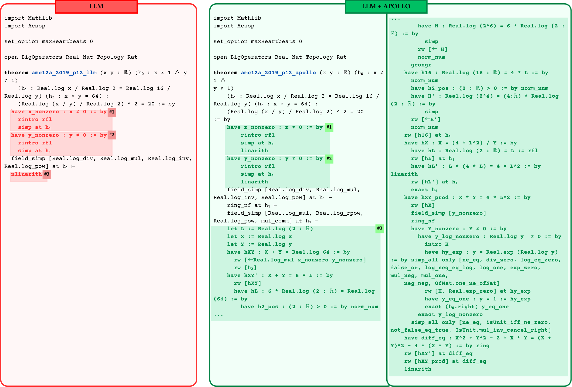
The image displays a side-by-side comparison of two Lean 4 code blocks, each attempting to prove the same mathematical theorem (`amc12a_2019_p12`). The left block, outlined in red and labeled "LLM," shows a shorter, more direct proof attempt. The right block, outlined in green and labeled "LLM + APOLLO," shows a longer, more detailed proof that introduces intermediate variables and lemmas. The comparison likely illustrates the difference in proof strategy or capability between a base Large Language Model (LLM) and an LLM augmented with a system named "APOLLO."
### Components/Axes
The image is structured as two vertical panels:
1. **Left Panel (LLM):**
* **Header:** A red rectangular label at the top center containing the text "LLM".
* **Border:** A red rounded rectangle enclosing the code.
* **Content:** Lean 4 code with specific lines highlighted in a light red/pink background. Annotations `#1`, `#2`, and `#3` are placed next to certain lines.
2. **Right Panel (LLM + APOLLO):**
* **Header:** A green rectangular label at the top center containing the text "LLM + APOLLO".
* **Border:** A green rounded rectangle enclosing the code.
* **Content:** Lean 4 code with a light green background. The code is more extensive. Annotations `#1`, `#2`, and `#3` are also present, corresponding to similar logical steps as in the left panel. The code continues beyond the visible frame, indicated by an ellipsis (`...`) at the top and bottom.
### Detailed Analysis
**Theorem Statement (Common to Both):**
Both blocks begin with identical setup and theorem statements:
```lean
import Mathlib
import Aesop
set_option maxHeartbeats 0
open BigOperators Real Nat Topology Rat
theorem amc12a_2019_p12_... (x y : ℝ) (h₀ : x ≠ 1 ∧ y ≠ 1)
(h₁ : Real.log x / Real.log 2 = Real.log 16 / Real.log y) (h₂ : x * y = 64) :
(Real.log (x / y) / Real.log 2) ^ 2 = 20 := by
```
The theorem concerns real numbers `x` and `y`, with hypotheses about their logs and product, aiming to prove a specific equation involving the log of their ratio.
**Left Panel (LLM) Proof Steps:**
1. **`have x_nonzero : x ≠ 0 := by`** (Highlighted, annotated `#1`):
* `rintro rfl`
* `simp at h₁`
2. **`have y_nonzero : y ≠ 0 := by`** (Highlighted, annotated `#2`):
* `rintro rfl`
* `simp at h₁`
3. **`field_simp [Real.log_div, Real.log_mul, Real.log_inv, Real.log_pow] at h₁ ⊢`**
4. **`nlinarith`** (Highlighted, annotated `#3`)
**Right Panel (LLM + APOLLO) Proof Steps:**
The proof is more elaborate. Key differences and extensions include:
1. **`have x_nonzero : x ≠ 0 := by`** (Annotated `#1`):
* `rintro rfl`
* `simp at h₁`
* `linarith` (Uses a different tactic than the LLM version).
2. **`have y_nonzero : y ≠ 0 := by`** (Annotated `#2`):
* `rintro rfl`
* `simp at h₁`
* `linarith`
3. **`field_simp` and `ring_nf` tactics** are applied to `h₁`.
4. **Introduction of Intermediate Variables** (Annotated `#3`):
* `let L := Real.log (2 : ℝ)`
* `let X := Real.log x`
* `let Y := Real.log y`
5. **Derivation of Lemmas:** The proof then builds a chain of logical steps using these variables:
* `have hXY : X + Y = Real.log 64 := by ...`
* `have hXY' : X + Y = 6 * L := by ...`
* `have hL : 6 * Real.log (2 : ℝ) = Real.log (64) := by ...`
* `have h2_pos : (2 : ℝ) > 0 := by norm_num`
* (The code continues with more `have` statements, defining `h16`, `h2_pos`, `H'`, `hX`, `hL'`, `hXY_prod`, `Y_nonzero`, `y_log_nonzero`, `hy_exp`, `y_eq_one`, `diff_eq`, etc., before concluding with `linarith`).
### Key Observations
1. **Proof Strategy:** The LLM proof is concise, relying on `field_simp` and a single `nlinarith` call. The LLM + APOLLO proof is methodical, explicitly defining logarithmic substitutions (`L`, `X`, `Y`) and proving numerous intermediate equalities and properties.
2. **Tactic Usage:** The LLM version uses `nlinarith` (nonlinear arithmetic) at the end. The APOLLO version uses `linarith` (linear arithmetic) multiple times and employs more rewriting (`rw`) and simplification (`simp`) steps.
3. **Structure:** The APOLLO proof is highly structured, with each logical step isolated in a `have` block. This makes the proof more readable and verifiable but significantly longer.
4. **Annotations:** The `#1`, `#2`, `#3` annotations in both panels highlight analogous points in the proofs: establishing non-zero conditions (`#1`, `#2`) and the main proof strategy or variable introduction (`#3`).
### Interpretation
This diagram serves as a qualitative comparison of proof generation capabilities. It suggests that the "APOLLO" augmentation leads to a more **structured, explicit, and human-readable** proof style.
* **LLM Approach:** Represents a more direct, "black-box" style where complex tactics (`nlinarith`) are used to close the goal after some preprocessing. This is efficient but may be less instructive and harder to debug if it fails.
* **LLM + APOLLO Approach:** Represents a **decompositional** strategy. By introducing `L`, `X`, and `Y`, it transforms the problem about `x` and `y` into a problem about their logarithms, which is a standard technique for solving such equations. The extensive use of intermediate lemmas (`have` statements) breaks the proof into small, manageable, and self-contained steps. This mirrors how a human mathematician might structure the proof, enhancing transparency and trust in the result.
The key takeaway is not about the correctness of the theorem (which is the same in both), but about the **process and explainability** of the proof. The APOLLO-augmented system appears to prioritize generating a proof that is not just correct, but also **verifiable and pedagogically clear**, which is a crucial goal in automated reasoning and AI-assisted mathematics. The ellipsis (`...`) indicates the APOLLO proof is even longer than shown, further emphasizing its thoroughness.