## Line Graph: Convergence of Two Metrics with Sample Size
### Overview
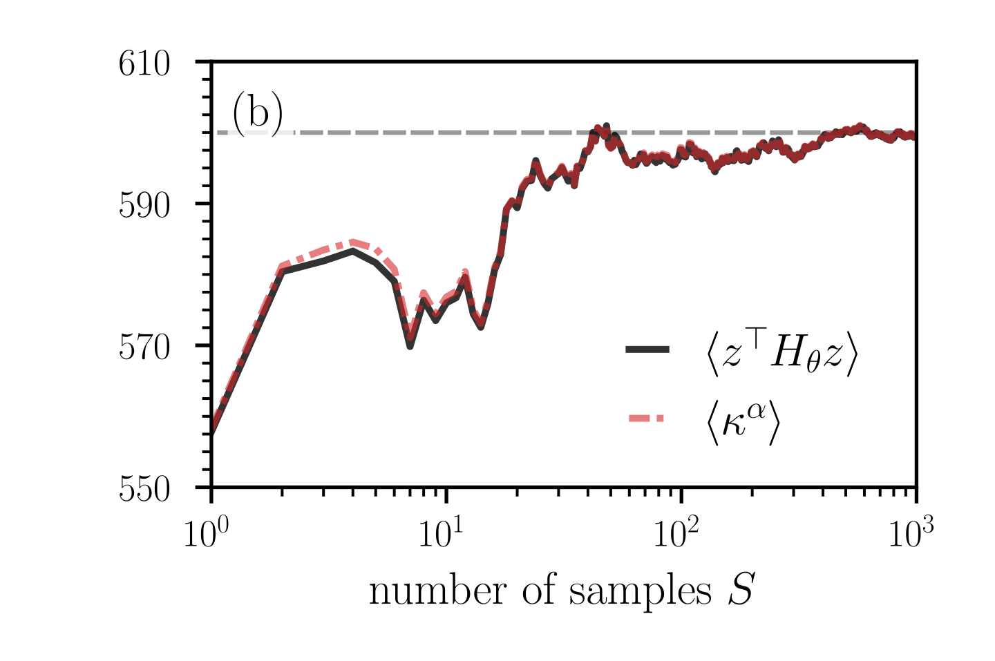
The image displays a scientific line graph, labeled "(b)" in the top-left corner, indicating it is likely part of a multi-panel figure. The graph plots the values of two distinct mathematical metrics against the number of samples, S, on a logarithmic scale. Both metrics show an initial rapid increase, followed by fluctuations, and eventual convergence toward a common asymptotic value.
### Components/Axes
* **X-Axis:**
* **Label:** `number of samples S`
* **Scale:** Logarithmic (base 10).
* **Range:** From `10^0` (1) to `10^3` (1000).
* **Major Ticks:** At `10^0`, `10^1`, `10^2`, `10^3`.
* **Minor Ticks:** Present between major ticks, indicating intermediate logarithmic values (e.g., 2, 3, 4... between 1 and 10).
* **Y-Axis:**
* **Label:** Not explicitly stated. The axis represents the numerical value of the plotted metrics.
* **Scale:** Linear.
* **Range:** From 550 to 610.
* **Major Ticks:** At 550, 570, 590, 610.
* **Minor Ticks:** Present, with 4 minor ticks between each major tick, representing increments of 4 units (e.g., 554, 558, 562, 566 between 550 and 570).
* **Legend:**
* **Position:** Bottom-right quadrant of the chart area.
* **Content:**
1. A solid black line segment followed by the text: `⟨z^T H_θ z⟩`
2. A dashed red line segment followed by the text: `⟨κ^α⟩`
* **Reference Line:** A horizontal, dashed gray line is present at approximately y = 600, spanning the width of the graph. This likely represents a theoretical limit, target, or asymptotic value.
### Detailed Analysis
**Data Series 1: `⟨z^T H_θ z⟩` (Solid Black Line)**
* **Trend Verification:** The line starts low, rises steeply, peaks, experiences a significant dip, recovers with fluctuations, and then stabilizes near the top of the graph.
* **Key Data Points (Approximate):**
* At S=1 (`10^0`): y ≈ 555.
* At S≈5: Reaches a local maximum of y ≈ 582.
* At S≈8: Drops to a local minimum of y ≈ 570.
* At S≈15: Another local minimum of y ≈ 573.
* From S≈20 to S≈50: Shows a steep, jagged increase.
* At S≈60: Reaches a peak near y ≈ 602, slightly above the dashed reference line.
* For S > 100: Oscillates with decreasing amplitude around y ≈ 600, closely following the dashed reference line.
**Data Series 2: `⟨κ^α⟩` (Dashed Red Line)**
* **Trend Verification:** Follows a very similar trajectory to the black line but with slightly less pronounced dips and peaks in the mid-range. It converges to the same final value.
* **Key Data Points (Approximate):**
* At S=1 (`10^0`): y ≈ 555 (nearly identical to the black line).
* At S≈5: Reaches a local maximum of y ≈ 585 (slightly higher than the black line).
* At S≈8: Dips to y ≈ 572 (less severe than the black line's dip).
* At S≈15: Dips to y ≈ 575.
* From S≈20 onward: Tracks the black line very closely, often overlapping.
* For S > 100: Converges and oscillates with the black line around y ≈ 600.
**Convergence Behavior:**
Both lines show high variance for sample sizes between S=1 and S≈100. For S > 100, the fluctuations diminish significantly, and both metrics stabilize near the value of 600, as indicated by the dashed gray reference line.
### Key Observations
1. **Strong Correlation:** The two metrics `⟨z^T H_θ z⟩` and `⟨κ^α⟩` are highly correlated across the entire range of sample sizes. Their trajectories are nearly identical, especially for S > 20.
2. **Initial Volatility:** The most significant fluctuations and the largest divergence between the two lines occur at low sample counts (S < 20).
3. **Asymptotic Convergence:** Both metrics appear to converge to a common value of approximately 600 as the number of samples increases beyond 100. The dashed gray line at y=600 serves as a visual guide for this limit.
4. **Logarithmic Scale Insight:** The use of a logarithmic x-axis emphasizes the behavior at small sample sizes, revealing the detailed structure of the initial rise and fluctuations that would be compressed on a linear scale.
### Interpretation
This graph demonstrates the convergence of two different estimators or quantities, `⟨z^T H_θ z⟩` and `⟨κ^α⟩`, as the sample size `S` increases. The notation suggests these are expected values (angle brackets `⟨ ⟩`) involving mathematical objects like vectors (`z`), matrices (`H_θ`), and exponents (`α`).
The key takeaway is that both quantities are consistent estimators: they approach the same true value (≈600) with increasing data. The initial volatility indicates high variance in the estimates when data is scarce. The fact that the two distinct mathematical expressions converge to the same limit suggests they may be theoretically equivalent or are measuring the same underlying property of the system being studied. The dashed line at 600 likely represents the known or theoretical asymptotic value, confirming the estimators' accuracy in the large-sample limit. The plot validates that a sample size of S > 100 is sufficient for both metrics to provide stable and reliable estimates.