## Diagram: Comparison of Activation-Based vs. Hidden state-Based Sequential Processing Architectures
### Overview
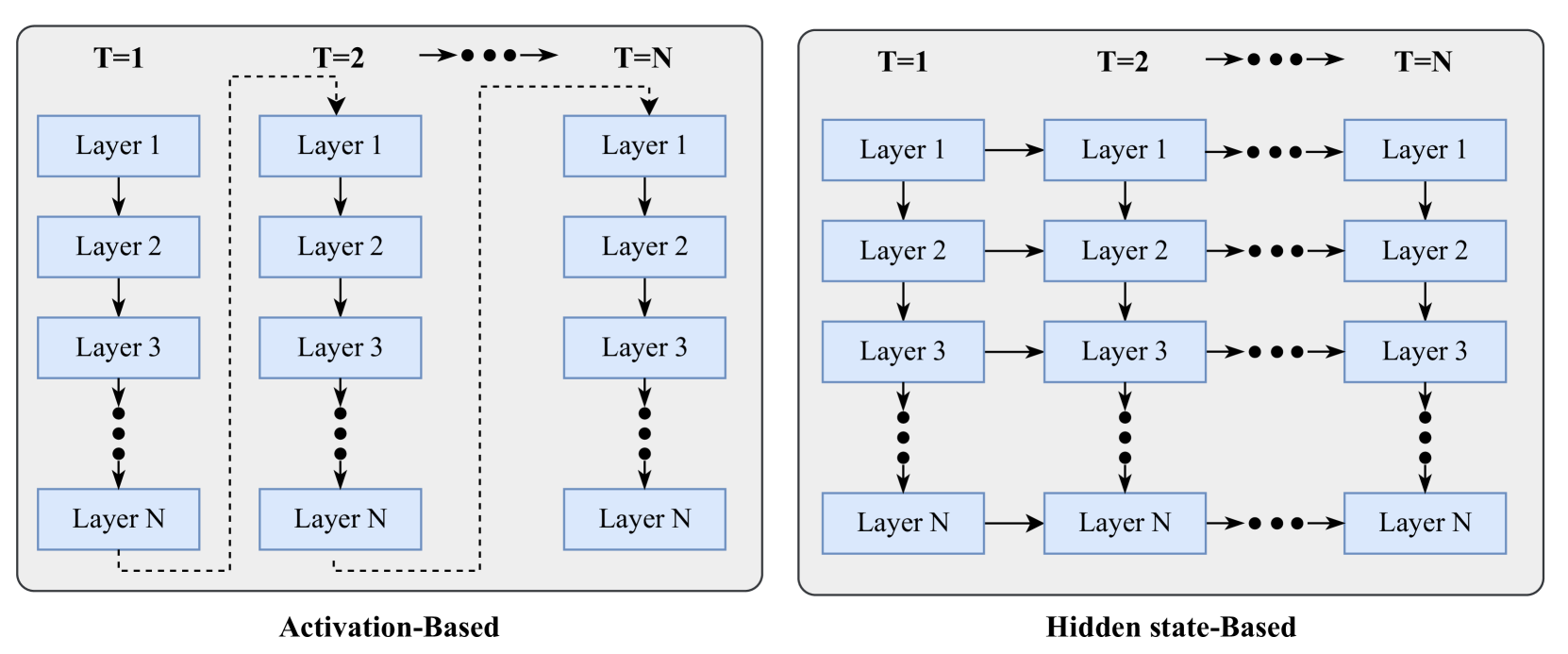
The image displays two side-by-side schematic diagrams illustrating two different architectural paradigms for processing sequential data (e.g., time series, language) through a deep neural network with multiple layers. The left diagram is titled "Activation-Based," and the right diagram is titled "Hidden state-Based." Both diagrams depict processing across discrete time steps (T=1, T=2, ..., T=N) and through a stack of layers (Layer 1 to Layer N).
### Components/Axes
**Common Elements in Both Diagrams:**
* **Time Steps:** Represented horizontally across the top. Labels are "T=1", "T=2", and "T=N", with an ellipsis ("•••") and an arrow between T=2 and T=N, indicating a sequence of intermediate steps.
* **Layers:** Represented vertically. Each time step contains a column of rectangular boxes labeled "Layer 1", "Layer 2", "Layer 3", followed by a vertical ellipsis ("⋮"), and finally "Layer N". This indicates a deep network with N layers.
* **Flow Arrows:** Solid black arrows indicate the direction of data or information flow.
**Diagram-Specific Elements:**
* **Left Panel (Activation-Based):**
* **Title:** "Activation-Based" is centered below the diagram.
* **Vertical Flow:** Within each time step column, arrows point downward from Layer 1 to Layer 2, Layer 2 to Layer 3, and so on, culminating at Layer N.
* **Temporal Connection:** A dashed line originates from the bottom of the "Layer N" box at T=1, travels right, then up, and connects to the top of the "Layer 1" box at T=2. A similar dashed line connects Layer N at T=2 to Layer 1 at T=N. This pattern implies the final output (activation) of the entire network at one time step is fed as the input to the first layer of the next time step.
* **Right Panel (Hidden state-Based):**
* **Title:** "Hidden state-Based" is centered below the diagram.
* **Vertical Flow:** Identical to the left panel; arrows point downward through the layers within each time step.
* **Temporal Connection:** Solid horizontal arrows connect corresponding layers across time steps. An arrow points from "Layer 1" at T=1 to "Layer 1" at T=2, and from "Layer 1" at T=2 to "Layer 1" at T=N (with ellipsis). This pattern repeats for Layer 2, Layer 3, and Layer N. This implies that the hidden state of each individual layer is passed directly to the same layer in the next time step.
### Detailed Analysis
**Activation-Based Flow (Left Diagram):**
1. **Intra-step Processing:** At time T=1, input enters Layer 1. The output of Layer 1 becomes the input to Layer 2, and this process continues sequentially down to Layer N.
2. **Inter-step Handoff:** The final activation from Layer N at T=1 is used as the input for Layer 1 at T=2. The network's complete processing for one time step must finish before the next step begins.
3. **Pattern:** The flow is strictly serial across time, with a full forward pass through all N layers required for each time step. The dashed lines emphasize that the connection between time steps occurs only at the network's final output.
**Hidden state-Based Flow (Right Diagram):**
1. **Intra-step Processing:** Identical to the left diagram; data flows down through the layers within a single time step.
2. **Inter-step Handoff:** Concurrently with the vertical flow, each layer maintains and passes its own state horizontally. The hidden state of Layer 1 at T=1 is sent to Layer 1 at T=2. The hidden state of Layer 2 at T=1 is sent to Layer 2 at T=2, and so forth for all layers.
3. **Pattern:** This allows for parallel processing across time at the layer level. Information from past time steps is directly accessible to each layer, not just through the final network output. The solid horizontal arrows indicate a persistent, layer-specific memory.
### Key Observations
1. **Structural Difference:** The core distinction is the point of temporal connection. Activation-Based connects the *final output* of the network across time. Hidden state-Based connects the *intermediate states* of each layer across time.
2. **Information Bottleneck:** The Activation-Based model creates a potential bottleneck, as all temporal information must be compressed into the single vector output by Layer N before being passed to the next step.
3. **Parallelism Potential:** The Hidden state-Based architecture suggests a design where computations for different time steps can be more parallelized, as each layer's state is updated independently based on its own previous state and the current input from the layer below.
4. **Visual Emphasis:** The use of dashed lines for temporal connections in the Activation-Based diagram versus solid lines in the Hidden state-Based diagram visually reinforces the difference between an indirect, post-processing connection and a direct, stateful connection.
### Interpretation
These diagrams illustrate two fundamental approaches to modeling temporal dependencies in deep learning, commonly seen in Recurrent Neural Networks (RNNs) and their variants.
* **Activation-Based** is characteristic of a standard **vanilla RNN** or a **sequence-to-sequence model without skip connections**. The entire network processes one input vector to produce one output vector, which is then fed back as input for the next step. This can make learning long-term dependencies difficult due to vanishing/exploding gradients over many time steps, as the error signal must backpropagate through the entire depth of the network for each step.
* **Hidden state-Based** is characteristic of architectures like the **Long Short-Term Memory (LSTM)** or **Gated Recurrent Unit (GRU)** network, and is a foundational concept for **Residual Networks (ResNets) applied to sequences**. By maintaining and passing a hidden state at each layer, the network creates "shortcuts" for information flow across time. This design mitigates the vanishing gradient problem, allows the model to learn which information to retain or forget at each layer, and enables more stable training of deep sequential models. The diagram suggests a more sophisticated and powerful mechanism for capturing temporal dynamics, where each level of abstraction (each layer) can maintain its own memory of the past.