## Line Chart: Per-Period Regret vs. Time Period (t)
### Overview
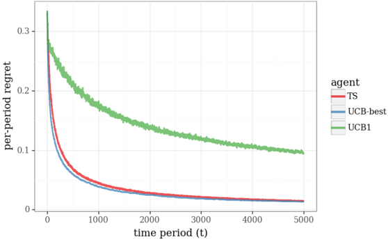
The image is a line chart comparing the performance of four different agents (algorithms) over time, measured by "per-period regret." The chart demonstrates how the regret metric decreases for all agents as the time period increases, but at significantly different rates and to different final levels.
### Components/Axes
* **Chart Type:** Line chart with multiple series.
* **Y-Axis:**
* **Label:** `per-period regret`
* **Scale:** Linear, ranging from 0 to approximately 0.33.
* **Major Ticks:** 0, 0.1, 0.2, 0.3.
* **X-Axis:**
* **Label:** `time period (t)`
* **Scale:** Linear, ranging from 0 to 5000.
* **Major Ticks:** 0, 1000, 2000, 3000, 4000, 5000.
* **Legend:**
* **Position:** Right side of the chart, vertically centered.
* **Title:** `agent`
* **Entries (from top to bottom):**
1. **TS** - Represented by a **red** line.
2. **UCB-best** - Represented by a **blue** line.
3. **UCB1** - Represented by a **green** line.
4. **UCB** - Represented by a **gray** line.
### Detailed Analysis
The chart plots four distinct data series, each showing a decaying trend.
1. **TS (Red Line):**
* **Trend:** Starts at a high regret value (~0.28 at t=0), decreases rapidly in an exponential-like decay, and then gradually flattens.
* **Key Points:** Crosses below 0.1 regret around t=500. By t=5000, the regret is very low, approximately 0.02.
2. **UCB-best (Blue Line):**
* **Trend:** Follows a path very similar to TS but consistently slightly lower. It also shows a rapid initial decay followed by a long tail.
* **Key Points:** Starts slightly lower than TS (~0.25 at t=0). Remains the lowest or second-lowest curve throughout. By t=5000, it converges to a value nearly identical to TS, around 0.02.
3. **UCB1 (Green Line):**
* **Trend:** Starts at the highest initial regret (~0.33 at t=0). Decays much more slowly than the other three agents, maintaining a significantly higher regret for the entire duration shown.
* **Key Points:** Remains above 0.2 until approximately t=800. At t=5000, its regret is still around 0.1, which is an order of magnitude higher than TS and UCB-best.
4. **UCB (Gray Line):**
* **Trend:** Starts at the lowest initial regret (~0.22 at t=0). Decays extremely rapidly, dropping below 0.05 before t=200. It then plateaus very close to zero.
* **Key Points:** Is the lowest curve for the first ~100 time periods. After t=1000, it is virtually indistinguishable from the x-axis (regret ≈ 0).
### Key Observations
* **Performance Hierarchy:** There is a clear and persistent separation in performance. From best (lowest regret) to worst (highest regret) for most of the timeline: **UCB (gray) ≈ UCB-best (blue) ≈ TS (red) << UCB1 (green)**.
* **Convergence:** The TS (red) and UCB-best (blue) lines converge to nearly the same low value by the end of the simulation (t=5000). The UCB (gray) line converges to near-zero much earlier.
* **Outlier:** The UCB1 (green) agent is a clear outlier, demonstrating substantially worse (higher) per-period regret throughout the entire observed period.
* **Initial Conditions:** The agents start at different regret levels, with UCB1 highest and UCB lowest.
### Interpretation
This chart likely visualizes the performance of different **multi-armed bandit algorithms**. "Regret" measures the difference between the reward gained by the algorithm and the reward that would have been gained by always choosing the optimal action. Lower regret is better.
* **What the data suggests:** The algorithms labeled **UCB**, **UCB-best**, and **TS** (likely Thompson Sampling) are highly effective, quickly learning to minimize regret. The standard **UCB1** algorithm, while also learning (regret decreases), is significantly less efficient in this specific scenario.
* **Relationship between elements:** The rapid initial drop in all curves indicates the "learning phase" where agents explore and identify better actions. The long, flat tails represent the "exploitation phase" where regret accumulates very slowly as the agents mostly choose the known optimal action. The proximity of the UCB-best and TS lines suggests these two advanced algorithms have comparable asymptotic performance here.
* **Notable Anomaly:** The stark underperformance of UCB1 compared to the other UCB variants (UCB, UCB-best) is the most striking finding. This could imply that the specific parameters or the variant of UCB used ("UCB" and "UCB-best") are much better tuned to the problem's characteristics (e.g., reward distribution, number of arms) than the standard UCB1 formulation. The chart makes a strong case for using more advanced bandit algorithms over the basic UCB1 in this context.