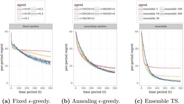
## Chart Type: Multiple Line Graphs Comparing Regret over Time ### Overview The image presents three line graphs comparing the per-period regret of different agents over time. Each graph represents a different exploration strategy: fixed epsilon-greedy, annealing epsilon-greedy, and ensemble Thompson Sampling (TS). The x-axis represents the time period (t), ranging from 0 to 500, and the y-axis represents the per-period regret, ranging from 0 to 60. Each graph plots multiple agents with different parameter settings for their respective exploration strategies. ### Components/Axes * **X-axis (all graphs):** time period (t), scale from 0 to 500 in increments of 100. * **Y-axis (all graphs):** per-period regret, scale from 0 to 60 in increments of 20. * **Graph Titles:** * (a) Fixed ε-greedy. * (b) Annealing ε-greedy. * (c) Ensemble TS. * **Legends (top-left of each graph):** Each legend identifies the agent type and its corresponding parameter settings. * **Fixed ε-greedy:** * Red: ε = 0.01 * Orange: ε = 0.05 * Green: ε = 0.1 * Light Blue: ε = 0.2 * Dark Blue: ε = 0.3 * **Annealing ε-greedy:** * Red: ε = 10/(10+t) * Orange: ε = 20/(20+t) * Green: ε = 30/(30+t) * Light Blue: ε = 40/(40+t) * Dark Blue: ε = 50/(50+t) * **Ensemble TS:** * Red: ensemble 3 * Orange: ensemble 10 * Green: ensemble 30 * Light Blue: ensemble 100 * Dark Blue: ensemble 300 ### Detailed Analysis #### (a) Fixed ε-greedy * **Trend:** The per-period regret generally decreases initially and then plateaus. The level at which it plateaus depends on the epsilon value. * **Data Points:** * ε = 0.01 (Red): Starts around 60, decreases to approximately 38, and remains relatively constant. * ε = 0.05 (Orange): Starts around 60, decreases to approximately 32, and remains relatively constant. * ε = 0.1 (Green): Starts around 60, decreases to approximately 25, and remains relatively constant. * ε = 0.2 (Light Blue): Starts around 60, decreases to approximately 23, and remains relatively constant. * ε = 0.3 (Dark Blue): Starts around 60, decreases to approximately 22, and remains relatively constant. #### (b) Annealing ε-greedy * **Trend:** The per-period regret decreases over time for all agents. * **Data Points:** * ε = 10/(10+t) (Red): Starts around 60, decreases to approximately 15. * ε = 20/(20+t) (Orange): Starts around 60, decreases to approximately 13. * ε = 30/(30+t) (Green): Starts around 60, decreases to approximately 12. * ε = 40/(40+t) (Light Blue): Starts around 60, decreases to approximately 11. * ε = 50/(50+t) (Dark Blue): Starts around 60, decreases to approximately 10. #### (c) Ensemble TS * **Trend:** The per-period regret decreases over time, with the ensemble size affecting the rate and final regret level. * **Data Points:** * Ensemble 3 (Red): Starts around 60, decreases to approximately 18, and remains relatively constant. * Ensemble 10 (Orange): Starts around 60, decreases to approximately 15, and remains relatively constant. * Ensemble 30 (Green): Starts around 60, decreases to approximately 12, and remains relatively constant. * Ensemble 100 (Light Blue): Starts around 60, decreases to approximately 10, and remains relatively constant. * Ensemble 300 (Dark Blue): Starts around 60, decreases to approximately 9, and remains relatively constant. ### Key Observations * In the fixed epsilon-greedy strategy, higher epsilon values lead to lower final regret levels but potentially slower initial learning. * The annealing epsilon-greedy strategy consistently reduces regret over time, regardless of the initial epsilon parameter. * In the ensemble TS strategy, larger ensemble sizes result in lower final regret levels. ### Interpretation The graphs demonstrate the impact of different exploration strategies on per-period regret. The fixed epsilon-greedy method balances exploration and exploitation, with the epsilon value controlling this balance. The annealing epsilon-greedy method dynamically adjusts the exploration rate, leading to continuous improvement. The ensemble TS method leverages multiple models to make decisions, with larger ensembles generally performing better. The data suggests that for this particular problem, annealing epsilon-greedy and ensemble TS are more effective at minimizing regret over time compared to fixed epsilon-greedy. The ensemble TS method with larger ensemble sizes appears to be the most effective strategy.

\n ## Line Charts: Per-Period Regret vs. Time Period for Different Agent Configurations ### Overview The image presents three line charts, labeled (a) Fixed ε-greedy, (b) Annealing ε-greedy, and (c) Ensemble TS. Each chart depicts the relationship between per-period regret (y-axis) and time period (t) (x-axis) for different agent configurations. The charts compare the performance of various parameter settings within each agent type. ### Components/Axes * **X-axis:** Time period (t), ranging from approximately 0 to 500. * **Y-axis:** Per-period regret, ranging from approximately 0 to 60. * **Chart (a) - Fixed ε-greedy:** * Legend: * ε = 0.01 (Pink) * ε = 0.05 (Green) * ε = 0.1 (Purple) * ε = 0.2 (Orange) * ε = 0.3 (Brown) * **Chart (b) - Annealing ε-greedy:** * Legend: * ε = 10/(10+t) (Pink) * ε = 20/(20+t) (Green) * ε = 30/(30+t) (Purple) * ε = 40/(40+t) (Orange) * ε = 50/(50+t) (Brown) * **Chart (c) - Ensemble TS:** * Legend: * ensemble 3 (Pink) * ensemble 10 (Green) * ensemble 30 (Purple) * ensemble 100 (Orange) * ensemble 300 (Brown) ### Detailed Analysis or Content Details **Chart (a) - Fixed ε-greedy:** * The pink line (ε = 0.01) starts at approximately 55 and decreases rapidly to around 10 by t=100, then plateaus around 8-10. * The green line (ε = 0.05) starts at approximately 55 and decreases to around 15 by t=100, then plateaus around 12-14. * The purple line (ε = 0.1) starts at approximately 55 and decreases to around 20 by t=100, then plateaus around 16-18. * The orange line (ε = 0.2) starts at approximately 55 and decreases to around 25 by t=100, then plateaus around 20-22. * The brown line (ε = 0.3) starts at approximately 55 and decreases to around 30 by t=100, then plateaus around 25-27. * All lines exhibit a decreasing trend, but the rate of decrease varies with ε. Lower ε values result in faster initial decreases and lower final regret values. **Chart (b) - Annealing ε-greedy:** * The pink line (ε = 10/(10+t)) starts at approximately 55 and decreases rapidly to around 8 by t=100, then continues to decrease slowly, reaching around 5 by t=500. * The green line (ε = 20/(20+t)) starts at approximately 55 and decreases rapidly to around 12 by t=100, then continues to decrease slowly, reaching around 8 by t=500. * The purple line (ε = 30/(30+t)) starts at approximately 55 and decreases rapidly to around 16 by t=100, then continues to decrease slowly, reaching around 11 by t=500. * The orange line (ε = 40/(40+t)) starts at approximately 55 and decreases rapidly to around 20 by t=100, then continues to decrease slowly, reaching around 14 by t=500. * The brown line (ε = 50/(50+t)) starts at approximately 55 and decreases rapidly to around 24 by t=100, then continues to decrease slowly, reaching around 17 by t=500. * Similar to Chart (a), all lines decrease over time, but the rate of decrease is influenced by the annealing schedule. **Chart (c) - Ensemble TS:** * The pink line (ensemble 3) starts at approximately 55 and decreases rapidly to around 10 by t=100, then plateaus around 6-8. * The green line (ensemble 10) starts at approximately 55 and decreases rapidly to around 8 by t=100, then plateaus around 5-7. * The purple line (ensemble 30) starts at approximately 55 and decreases rapidly to around 7 by t=100, then plateaus around 4-6. * The orange line (ensemble 100) starts at approximately 55 and decreases rapidly to around 6 by t=100, then plateaus around 3-5. * The brown line (ensemble 300) starts at approximately 55 and decreases rapidly to around 5 by t=100, then plateaus around 2-4. * All lines exhibit a decreasing trend, with larger ensemble sizes generally leading to lower regret values. ### Key Observations * In all three charts, the per-period regret decreases over time, indicating learning and improvement in the agents' performance. * Chart (c) (Ensemble TS) consistently shows the lowest regret values across all ensemble sizes, suggesting that ensemble methods are more effective at minimizing regret. * In Chart (a) (Fixed ε-greedy), lower ε values lead to better performance (lower regret). * In Chart (b) (Annealing ε-greedy), the initial rate of exploration decreases as time progresses, leading to a gradual reduction in regret. ### Interpretation The data suggests that the choice of agent configuration significantly impacts the per-period regret. Ensemble methods (Chart c) consistently outperform both fixed and annealing ε-greedy approaches. Within the fixed ε-greedy approach (Chart a), a lower exploration rate (lower ε) leads to better performance, but may also result in slower initial learning. The annealing ε-greedy approach (Chart b) provides a balance between exploration and exploitation, allowing the agent to adapt its exploration rate over time. The consistent downward trend in all charts indicates that the agents are learning from their experiences and improving their decision-making over time. The ensemble methods likely benefit from averaging out the predictions of multiple agents, reducing the variance and improving the overall performance. The plateaus observed in the later stages of the charts suggest that the agents have converged to a near-optimal policy.

## Multi-Panel Chart: Reinforcement Learning Agent Performance Comparison ### Overview The image displays three side-by-side line charts comparing the performance of different reinforcement learning agent strategies over 500 time periods. The performance metric is "per-period regret," where lower values indicate better performance. Each chart represents a distinct strategy: (a) Fixed ε-greedy, (b) Annealing ε-greedy, and (c) Ensemble Thompson Sampling (TS). ### Components/Axes * **Common Elements Across All Charts:** * **Y-axis:** Label: `per-period regret`. Scale: 0 to 60, with major ticks at 0, 20, 40, 60. * **X-axis:** Label: `time period (t)`. Scale: 0 to 500, with major ticks at 0, 100, 200, 300, 400, 500. * **Legend Position:** Top-left corner within each chart's plotting area. * **Chart Titles (within gray bars):** (a) `fixed epsilon`, (b) `annealing epsilon`, (c) `ensemble`. * **Sub-captions:** (a) `Fixed ε-greedy.`, (b) `Annealing ε-greedy.`, (c) `Ensemble TS.` * **Chart-Specific Legends:** * **(a) Fixed ε-greedy:** * `agent` (header) * `ε=0.01` (red line) * `ε=0.05` (orange line) * `ε=0.1` (green line) * `ε=0.2` (light blue line) * `ε=0.3` (dark blue line) * **(b) Annealing ε-greedy:** * `agent` (header) * `ε=10/(10+t)` (red line) * `ε=20/(20+t)` (orange line) * `ε=30/(30+t)` (green line) * `ε=40/(40+t)` (light blue line) * `ε=50/(50+t)` (dark blue line) * **(c) Ensemble TS:** * `agent` (header) * `ensemble 3` (red line) * `ensemble 10` (orange line) * `ensemble 30` (green line) * `ensemble 100` (light blue line) * `ensemble 300` (dark blue line) ### Detailed Analysis **Chart (a): Fixed ε-greedy** * **Trend:** All lines show a decreasing trend in per-period regret over time, starting near 60 and declining. The rate of decline and final plateau level differ by ε value. * **Data Series & Approximate Values:** * `ε=0.01` (red): Declines slowly, plateaus highest at approximately 38-40 regret by t=500. * `ε=0.05` (orange): Declines moderately, plateaus around 30-32 regret. * `ε=0.1` (green): Declines more steeply, plateaus around 25-27 regret. * `ε=0.2` (light blue): Declines steeply, plateaus around 22-24 regret. * `ε=0.3` (dark blue): Declines most steeply initially, plateaus lowest at approximately 20-22 regret. * **Observation:** Higher fixed ε values (more exploration) lead to faster initial regret reduction and a lower final regret plateau in this 500-period window. **Chart (b): Annealing ε-greedy** * **Trend:** All lines show a steep, smooth decline in regret, converging more tightly than in chart (a). * **Data Series & Approximate Values:** * All five lines (`ε=10/(10+t)` to `ε=50/(50+t)`) follow very similar trajectories. * They start near 60 regret and decline rapidly, beginning to plateau around t=300. * By t=500, all lines are clustered in a narrow band between approximately 12-18 regret. The line for `ε=10/(10+t)` (red) appears to plateau slightly higher (~18) than the others (~12-15). * **Observation:** The annealing (decaying) exploration rate leads to strong, consistent performance across different initial parameters, with all variants achieving lower final regret than the best fixed ε strategy. **Chart (c): Ensemble TS** * **Trend:** All lines show a very steep initial decline in regret, followed by a plateau. The performance gap between ensemble sizes is distinct. * **Data Series & Approximate Values:** * `ensemble 3` (red): Declines but plateaus significantly higher than others, at approximately 18-20 regret. * `ensemble 10` (orange): Plateaus around 8-10 regret. * `ensemble 30` (green): Plateaus around 4-6 regret. * `ensemble 100` (light blue): Plateaus very low, around 2-4 regret. * `ensemble 300` (dark blue): Plateaus the lowest, approaching 0-2 regret. * **Observation:** There is a clear, monotonic relationship: larger ensemble sizes lead to dramatically lower per-period regret. The performance improvement from ensemble 3 to ensemble 300 is substantial. ### Key Observations 1. **Performance Hierarchy:** Across the strategies shown at t=500, Ensemble TS with large ensembles (100, 300) achieves the lowest regret (~0-4), followed by Annealing ε-greedy (~12-18), then the best Fixed ε-greedy (~20-22), with the worst being small ensembles or low fixed ε. 2. **Convergence Speed:** Ensemble TS and Annealing ε-greedy show faster initial convergence (steeper slopes) compared to Fixed ε-greedy. 3. **Parameter Sensitivity:** Fixed ε-greedy is highly sensitive to the chosen ε value. Annealing ε-greedy is robust to its initial parameter. Ensemble TS performance scales directly and strongly with ensemble size. 4. **Visual Clustering:** In charts (b) and (c), the lines for better-performing parameters (higher annealing constants, larger ensembles) are tightly clustered at the bottom of the chart. ### Interpretation This set of charts demonstrates a comparative analysis of exploration strategies in a simulated reinforcement learning environment. The "per-period regret" metric quantifies the cost of not choosing the optimal action at each time step. * **Fixed ε-greedy** represents a static exploration strategy. The data suggests that in this specific problem, a higher constant exploration rate (ε=0.3) is beneficial over 500 steps, as it allows the agent to discover good actions faster, outweighing the cost of random exploration. However, its performance is ultimately limited. * **Annealing ε-greedy** implements a dynamic strategy where exploration decreases over time. The tight clustering of results indicates this approach is **robust**; it performs well across a range of decay schedules. It outperforms the static strategy because it balances early exploration with later exploitation effectively. * **Ensemble Thompson Sampling** is a more sophisticated, probabilistic approach that maintains multiple hypotheses (an ensemble) about the environment. The clear, monotonic improvement with ensemble size indicates that **increased model complexity (more ensemble members) directly translates to better decision-making and lower regret** in this context. It is the most effective strategy shown, with large ensembles nearly eliminating regret. **Underlying Message:** The visualization argues for the superiority of adaptive (annealing) and probabilistic (ensemble) exploration strategies over static ones for this class of problem. It also highlights a key trade-off: computational cost (larger ensembles) yields significant performance gains. The charts provide empirical evidence to guide algorithm selection and hyperparameter tuning.

## Line Graphs: Per-Period Regret Over Time Periods ### Overview The image contains three line graphs comparing per-period regret across different time periods (t) for three strategies: (a) Fixed ε-greedy, (b) Annealing ε-greedy, and (c) Ensemble TS. Each graph shows multiple data series with distinct colors, representing variations in parameters (ε-values for ε-greedy strategies, ensemble sizes for TS). All graphs share identical axes: y-axis labeled "per-period regret" (0–60) and x-axis labeled "time period (t)" (0–500). --- ### Components/Axes 1. **Graph Titles**: - (a) Fixed ε-greedy - (b) Annealing ε-greedy - (c) Ensemble TS 2. **Axes**: - **Y-axis**: "per-period regret" (0–60, linear scale). - **X-axis**: "time period (t)" (0–500, linear scale). 3. **Legends**: - **(a) Fixed ε-greedy**: - Colors: Red (ε=0.01), Teal (ε=0.2), Orange (ε=0.05), Purple (ε=0.3), Green (ε=0.1). - **(b) Annealing ε-greedy**: - Colors: Red (ε=10/(10+t)), Teal (ε=40/(40+t)), Orange (ε=20/(20+t)), Purple (ε=50/(50+t)), Green (ε=30/(30+t)). - **(c) Ensemble TS**: - Colors: Red (ensemble 3), Teal (ensemble 100), Orange (ensemble 10), Purple (ensemble 300), Green (ensemble 30). 4. **Legend Placement**: - All legends are positioned at the top of their respective graphs, with labels aligned left-to-right. --- ### Detailed Analysis #### (a) Fixed ε-greedy - **Trends**: All lines start near 60 regret and decrease over time. Lower ε-values (e.g., ε=0.01, red) decline more sharply, while higher ε-values (e.g., ε=0.3, purple) decrease more gradually. - **Key Data Points**: - At t=500: - ε=0.01 (red): ~25 regret. - ε=0.3 (purple): ~35 regret. - ε=0.1 (green) and ε=0.2 (teal) converge to ~28–30 regret. #### (b) Annealing ε-greedy - **Trends**: Lines start higher (~60 regret) and decline more gradually than fixed ε-greedy. Annealing schedules (e.g., ε=10/(10+t)) show slower decay due to time-dependent ε reduction. - **Key Data Points**: - At t=500: - ε=10/(10+t) (red): ~30 regret. - ε=50/(50+t) (purple): ~35 regret. - ε=30/(30+t) (green) stabilizes near ~28 regret. #### (c) Ensemble TS - **Trends**: Lines start near 60 regret and drop sharply initially, then plateau. Larger ensembles (e.g., 300, purple) achieve lower regret faster than smaller ones (e.g., 3, red). - **Key Data Points**: - At t=500: - Ensemble 3 (red): ~20 regret. - Ensemble 300 (purple): ~10 regret. - Ensemble 100 (teal) and 30 (green) converge to ~12–15 regret. --- ### Key Observations 1. **Fixed ε-greedy**: Lower ε-values (more greedy) achieve lower regret faster, but higher ε-values (more exploratory) stabilize at higher regret. 2. **Annealing ε-greedy**: Time-dependent ε reduction slows regret decline compared to fixed ε-greedy, suggesting adaptive exploration improves long-term performance. 3. **Ensemble TS**: Larger ensembles (e.g., 300) outperform smaller ones, with regret dropping sharply initially and stabilizing at lower values. --- ### Interpretation The data demonstrates that exploration-exploitation trade-offs (via ε-greedy strategies) and ensemble diversity (via TS) significantly impact regret minimization. Fixed ε-greedy with low ε (e.g., 0.01) achieves the lowest regret but risks under-exploration. Annealing ε-greedy balances exploration over time, while Ensemble TS leverages diversity to reduce regret more effectively. Larger ensembles (e.g., 300) outperform smaller ones, highlighting the value of model aggregation. The sharp initial drops in Ensemble TS suggest rapid learning from diverse models, while annealing strategies adapt exploration dynamically.