## Chart Type: Multiple Line Graphs Comparing Regret over Time
### Overview
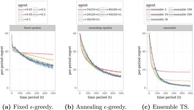
The image presents three line graphs comparing the per-period regret of different agents over time. Each graph represents a different exploration strategy: fixed epsilon-greedy, annealing epsilon-greedy, and ensemble Thompson Sampling (TS). The x-axis represents the time period (t), ranging from 0 to 500, and the y-axis represents the per-period regret, ranging from 0 to 60. Each graph plots multiple agents with different parameter settings for their respective exploration strategies.
### Components/Axes
* **X-axis (all graphs):** time period (t), scale from 0 to 500 in increments of 100.
* **Y-axis (all graphs):** per-period regret, scale from 0 to 60 in increments of 20.
* **Graph Titles:**
* (a) Fixed ε-greedy.
* (b) Annealing ε-greedy.
* (c) Ensemble TS.
* **Legends (top-left of each graph):** Each legend identifies the agent type and its corresponding parameter settings.
* **Fixed ε-greedy:**
* Red: ε = 0.01
* Orange: ε = 0.05
* Green: ε = 0.1
* Light Blue: ε = 0.2
* Dark Blue: ε = 0.3
* **Annealing ε-greedy:**
* Red: ε = 10/(10+t)
* Orange: ε = 20/(20+t)
* Green: ε = 30/(30+t)
* Light Blue: ε = 40/(40+t)
* Dark Blue: ε = 50/(50+t)
* **Ensemble TS:**
* Red: ensemble 3
* Orange: ensemble 10
* Green: ensemble 30
* Light Blue: ensemble 100
* Dark Blue: ensemble 300
### Detailed Analysis
#### (a) Fixed ε-greedy
* **Trend:** The per-period regret generally decreases initially and then plateaus. The level at which it plateaus depends on the epsilon value.
* **Data Points:**
* ε = 0.01 (Red): Starts around 60, decreases to approximately 38, and remains relatively constant.
* ε = 0.05 (Orange): Starts around 60, decreases to approximately 32, and remains relatively constant.
* ε = 0.1 (Green): Starts around 60, decreases to approximately 25, and remains relatively constant.
* ε = 0.2 (Light Blue): Starts around 60, decreases to approximately 23, and remains relatively constant.
* ε = 0.3 (Dark Blue): Starts around 60, decreases to approximately 22, and remains relatively constant.
#### (b) Annealing ε-greedy
* **Trend:** The per-period regret decreases over time for all agents.
* **Data Points:**
* ε = 10/(10+t) (Red): Starts around 60, decreases to approximately 15.
* ε = 20/(20+t) (Orange): Starts around 60, decreases to approximately 13.
* ε = 30/(30+t) (Green): Starts around 60, decreases to approximately 12.
* ε = 40/(40+t) (Light Blue): Starts around 60, decreases to approximately 11.
* ε = 50/(50+t) (Dark Blue): Starts around 60, decreases to approximately 10.
#### (c) Ensemble TS
* **Trend:** The per-period regret decreases over time, with the ensemble size affecting the rate and final regret level.
* **Data Points:**
* Ensemble 3 (Red): Starts around 60, decreases to approximately 18, and remains relatively constant.
* Ensemble 10 (Orange): Starts around 60, decreases to approximately 15, and remains relatively constant.
* Ensemble 30 (Green): Starts around 60, decreases to approximately 12, and remains relatively constant.
* Ensemble 100 (Light Blue): Starts around 60, decreases to approximately 10, and remains relatively constant.
* Ensemble 300 (Dark Blue): Starts around 60, decreases to approximately 9, and remains relatively constant.
### Key Observations
* In the fixed epsilon-greedy strategy, higher epsilon values lead to lower final regret levels but potentially slower initial learning.
* The annealing epsilon-greedy strategy consistently reduces regret over time, regardless of the initial epsilon parameter.
* In the ensemble TS strategy, larger ensemble sizes result in lower final regret levels.
### Interpretation
The graphs demonstrate the impact of different exploration strategies on per-period regret. The fixed epsilon-greedy method balances exploration and exploitation, with the epsilon value controlling this balance. The annealing epsilon-greedy method dynamically adjusts the exploration rate, leading to continuous improvement. The ensemble TS method leverages multiple models to make decisions, with larger ensembles generally performing better. The data suggests that for this particular problem, annealing epsilon-greedy and ensemble TS are more effective at minimizing regret over time compared to fixed epsilon-greedy. The ensemble TS method with larger ensemble sizes appears to be the most effective strategy.