## Diagram: MCTS* and LLM Self-Training
### Overview
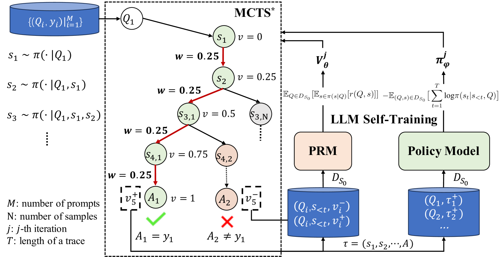
The image is a diagram illustrating a process involving Monte Carlo Tree Search (MCTS*) and Large Language Model (LLM) self-training. It shows the flow of data and interactions between different components, including prompts, states, actions, and models.
### Components/Axes
* **Top-Left**: A blue cylinder labeled "{(Qi, yi) | i=1 to M}". This represents a set of prompts and corresponding target outputs.
* **Left**: Text describing parameters:
* "M: number of prompts"
* "N: number of samples"
* "j: j-th iteration"
* "T: length of a trace"
* **Center**: A dashed-line box labeled "MCTS*". Inside this box is a tree-like structure representing the search process.
* Nodes are labeled as Q1, s1, s2, s3,1, s3,N, s4,1, s4,2, A1, A2.
* Each node 's' has an associated value 'v' (e.g., s1 has v=0, s2 has v=0.25, s3,1 has v=0.5, s4,1 has v=0.75, A1 has v=1).
* Edges connecting nodes have associated weights 'w' (all shown edges have w=0.25).
* The path from Q1 to A1 is highlighted in red.
* A1 has a green checkmark and the label "A1 = y1".
* A2 has a red "X" and the label "A2 ≠ y1".
* **Right**: "LLM Self-Training" section.
* Two blocks labeled "PRM" (salmon color) and "Policy Model" (light green).
* Two blue cylinders representing datasets: one labeled "(Qi, s<t, vi-), (Qi, s<t, vi+)" and the other labeled "(Q1, τ1+), (Q2, τ2+), ...".
* Arrows indicate the flow of data between these components.
* **Top-Right**: Two upward arrows labeled "Vθj" and "πφj".
* **Equations**:
* s1 ~ π(· | Q1)
* s2 ~ π(· | Q1, s1)
* s3 ~ π(· | Q1, s1, s2)
* E[Q ∈ D_S0] [E[s ∈ π(s|Q)] [r(Q, s)]] - E[(Q,s) ∈ D_S0] [Σ from t=1 to T log π(st | s<t, Q)]
* **Bottom**: τ = (s1, s2, ..., A)
### Detailed Analysis
* **MCTS* Tree**:
* The tree starts with node Q1.
* From Q1, there's a path to s1 (v=0), then to s2 (v=0.25), then to s3,1 (v=0.5), and finally to s4,1 (v=0.75).
* From s4,1, the path leads to A1 (v=1), which is marked as a correct action (A1 = y1).
* Another branch from s2 leads to s3,N, and from s3,1 to s4,2, and from s4,2 to A2, which is marked as an incorrect action (A2 ≠ y1).
* The weights 'w' on the edges are all 0.25.
* **LLM Self-Training**:
* The PRM (Prompt Retrieval Model) and Policy Model are central components.
* Both models use the dataset D_S0.
* The dataset contains tuples of (Q_i, s<t, v_i^-) and (Q_i, s<t, v_i^+).
* The Policy Model outputs (Q1, τ1+), (Q2, τ2+), where τ represents a trace (s1, s2, ..., A).
* **Equations**:
* The equations describe the sampling process for generating states (s1, s2, s3, ...).
* The equation involving expectations and summation represents a loss function or objective function used in the LLM self-training process.
### Key Observations
* The MCTS* tree explores different action sequences, with the red path representing a successful trace.
* The LLM self-training loop uses the PRM and Policy Model to refine the policy based on the generated traces.
* The values 'v' associated with the nodes in the MCTS* tree seem to represent some kind of score or reward.
* The weights 'w' on the edges are constant (0.25), suggesting a uniform exploration strategy.
### Interpretation
The diagram illustrates a reinforcement learning approach where an LLM is trained to generate correct actions in response to prompts. The MCTS* algorithm is used to explore the action space and identify promising traces. The LLM self-training loop uses the generated traces to update the policy model, improving its ability to generate correct actions. The PRM likely helps in retrieving relevant prompts or examples to guide the training process. The diagram highlights the interplay between exploration (MCTS*) and exploitation (LLM self-training) in this approach. The goal is to find a policy that maximizes the expected reward, as represented by the equation involving expectations and summation.