## Chart Analysis: Auditory Scene Statistics
### Overview
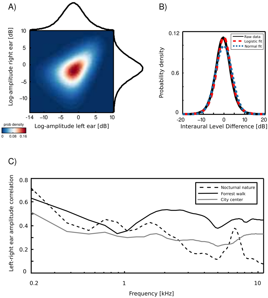
The image presents three plots (A, B, and C) analyzing auditory scene statistics. Plot A shows a 2D histogram of log-amplitude for the left and right ears, along with marginal distributions. Plot B displays the probability density of the interaural level difference, along with logistic and normal fits. Plot C shows the left-right ear amplitude correlation as a function of frequency for three different environments: nocturnal nature, forest walk, and city center.
### Components/Axes
**Plot A:**
* **Type:** 2D Histogram with Marginal Distributions
* **X-axis:** Log-amplitude left ear [dB]. Scale ranges from approximately -14 to 10.
* **Y-axis:** Log-amplitude right ear [dB]. Scale ranges from approximately -10 to 10.
* **Colorbar:** "prob density" ranging from 0 to 0.16. The color gradient goes from blue to red, with red indicating higher probability density.
* **Marginal Distributions:** Histograms along the x and y axes showing the distribution of log-amplitude for each ear independently.
**Plot B:**
* **Type:** Probability Density Plot
* **X-axis:** Interaural Level Difference [dB]. Scale ranges from -20 to 20.
* **Y-axis:** Probability density. Scale ranges from 0 to 0.12.
* **Legend (Top-Right):**
* Black line: Raw data
* Red dashed line: Logistic fit
* Blue dotted line: Normal fit
**Plot C:**
* **Type:** Line Plot
* **X-axis:** Frequency [kHz]. Logarithmic scale ranging from 0.2 to 10.
* **Y-axis:** Left-right ear amplitude correlation. Scale ranges from 0 to 0.8.
* **Legend (Top-Right):**
* Black dashed line: Nocturnal nature
* Black solid line: Forrest walk
* Gray solid line: City center
### Detailed Analysis
**Plot A:**
* The 2D histogram shows a positive correlation between the log-amplitude of the left and right ears. The highest probability density (red region) is centered around the origin (0,0), indicating that low amplitude sounds are most common.
* The marginal distributions show that the log-amplitudes for both ears are approximately normally distributed, centered around 0 dB.
**Plot B:**
* The raw data (black line) shows a distribution of interaural level differences centered around 0 dB.
* Both the logistic fit (red dashed line) and the normal fit (blue dotted line) closely approximate the raw data. The logistic fit appears to be slightly better at capturing the tails of the distribution.
**Plot C:**
* **Nocturnal nature (black dashed line):** Starts at approximately 0.7 correlation at 0.2 kHz, decreases to approximately 0.35 at 1 kHz, then increases to approximately 0.45 at 4 kHz, and decreases again to approximately 0.3 at 10 kHz.
* **Forrest walk (black solid line):** Starts at approximately 0.65 correlation at 0.2 kHz, decreases to approximately 0.35 at 1 kHz, increases to approximately 0.55 at 4 kHz, and remains relatively stable until 10 kHz.
* **City center (gray solid line):** Starts at approximately 0.5 correlation at 0.2 kHz, decreases to approximately 0.3 at 1 kHz, remains relatively stable until 4 kHz, and increases slightly to approximately 0.35 at 10 kHz.
### Key Observations
* Plot A shows a strong correlation between the log-amplitude of the left and right ears.
* Plot B indicates that the interaural level difference is approximately normally distributed.
* Plot C shows that the left-right ear amplitude correlation varies with frequency and is different for different environments. Nocturnal nature and forest walk environments have higher correlations at low frequencies compared to the city center.
### Interpretation
The plots provide insights into the statistical properties of auditory scenes. Plot A suggests that sounds are generally balanced between the left and right ears. Plot B indicates that the interaural level difference, which is important for sound localization, follows a predictable distribution. Plot C reveals that the correlation between the left and right ear amplitudes varies depending on the environment and frequency. This suggests that different environments have different spatial sound characteristics. The higher correlation at low frequencies in natural environments (nocturnal nature and forest walk) may be due to the presence of diffuse sound sources, while the lower correlation in the city center may be due to the presence of more localized sound sources.