## 3D Scatter Plots: Point Distribution in a Cube
### Overview
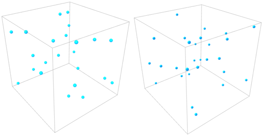
The image presents two 3D scatter plots, each contained within a wireframe cube. The plots display the spatial distribution of light blue spheres within the cubic volume. The left plot shows a more dispersed distribution, while the right plot exhibits a concentration of points towards the center of the cube.
### Components/Axes
* **Axes:** Each cube represents a 3D coordinate system, with the edges of the cube serving as the x, y, and z axes. The axes are not explicitly labeled with numerical values.
* **Data Points:** Light blue spheres represent the data points. The size of the spheres appears to vary slightly, but this variation does not seem to correlate with any specific axis or dimension.
* **Cube:** The cube is a wireframe, providing a visual boundary for the 3D space.
### Detailed Analysis
**Left Plot:**
* The light blue spheres are scattered throughout the volume of the cube.
* There is no apparent clustering or pattern in the distribution.
* The number of points is approximately 20-25.
**Right Plot:**
* The light blue spheres are concentrated towards the center of the cube.
* The density of points is higher in the central region compared to the edges and corners.
* The number of points is approximately 20-25.
### Key Observations
* The primary difference between the two plots is the spatial distribution of the points. The left plot shows a dispersed distribution, while the right plot shows a concentrated distribution.
* The size variation of the spheres is subtle and does not appear to encode any additional information.
* The cubes are identical in size and orientation.
### Interpretation
The image likely illustrates two different scenarios or datasets, where the spatial distribution of points within a 3D space is of interest. The left plot could represent a random or uniform distribution, while the right plot could represent a distribution with a central tendency. Without further context, it's difficult to determine the specific meaning of the data points or the axes. However, the image effectively conveys the concept of spatial distribution and the difference between dispersed and concentrated patterns.