## Multi-Panel Graph: Threshold and Difference Plots Across Signal Frequencies
### Overview
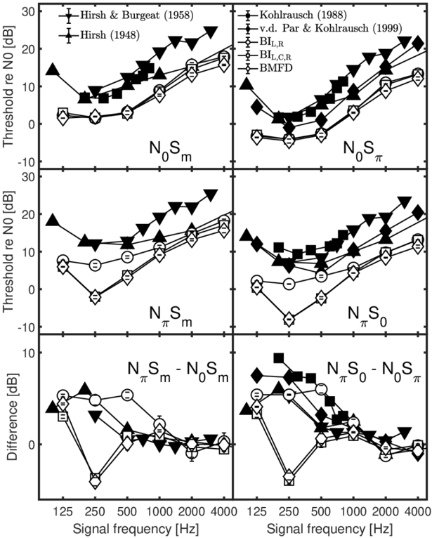
The image contains six subplots arranged in a 2x3 grid, comparing threshold values and differences across signal frequencies (125–4000 Hz). Each plot uses distinct symbols and lines to represent data from historical and modern studies (e.g., Hirsch & Burgeat 1958, Kohlrausch 1988). The graphs focus on relationships between noise thresholds (N₀), signal components (Sₘ, S₀, S_π), and their differences.
---
### Components/Axes
1. **X-Axes**:
- All plots share the same x-axis: **Signal frequency [Hz]** (125–4000 Hz).
- Subplots are labeled with terms like **N₀Sₘ**, **N₀S_π**, **N_πSₘ**, etc., indicating specific noise-signal relationships.
2. **Y-Axes**:
- **Top Row**: **Threshold re N₀ [dB]** (range: -30 to 30 dB).
- **Bottom Row**: **Difference [dB]** (range: -10 to 10 dB).
3. **Legends**:
- Positioned in the **top-right** of each plot.
- Symbols include:
- **Triangles** (▲): Hirsch & Burgeat (1958)
- **Squares** (■): Hirsch (1948)
- **Circles** (○): Kohlrausch (1988)
- **Diamonds** (◆): v.d. Par & Kohlrausch (1999)
- **Other symbols**: BI_L,R, BI_L,C,R, BMFDI (exact labels unclear due to resolution).
---
### Detailed Analysis
#### Top Row: Threshold Plots
1. **N₀Sₘ (Top-Left)**:
- **Trend**: All lines show an **upward trend** with increasing frequency.
- **Key Data**:
- Hirsch & Burgeat (1958): Peaks at ~2000 Hz (~25 dB).
- Hirsch (1948): Lower amplitude, peaks at ~1000 Hz (~15 dB).
- Kohlrausch (1988): Smooth rise, ~10 dB at 4000 Hz.
2. **N₀S_π (Top-Right)**:
- **Trend**: **Downward trend** at lower frequencies, then stabilizes.
- **Key Data**:
- v.d. Par & Kohlrausch (1999): Sharp drop to ~-10 dB at 500 Hz.
- BMFDI: Minimal variation, ~0 dB across frequencies.
#### Middle Row: Threshold Plots
3. **N_πSₘ (Middle-Left)**:
- **Trend**: **V-shaped** pattern (dips at ~1000 Hz).
- **Key Data**:
- BI_L,R: Lowest dip (~-5 dB at 1000 Hz).
- BI_L,C,R: Higher amplitude, ~5 dB at 2000 Hz.
4. **N_πS₀ (Middle-Right)**:
- **Trend**: **Upward trend** with frequency.
- **Key Data**:
- BMFDI: Steep rise, ~20 dB at 4000 Hz.
- Kohlrausch (1988): Gradual increase, ~15 dB at 2000 Hz.
#### Bottom Row: Difference Plots
5. **N_πSₘ - N₀Sₘ (Bottom-Left)**:
- **Trend**: **U-shaped** with minima at ~500 Hz.
- **Key Data**:
- Hirsch (1948): Sharp dip to ~-8 dB at 500 Hz.
- v.d. Par & Kohlrausch (1999): Shallow curve, ~-2 dB at 1000 Hz.
6. **N_πS₀ - N₀S_π (Bottom-Right)**:
- **Trend**: **Downward trend** with frequency.
- **Key Data**:
- BMFDI: Steep decline, ~-10 dB at 4000 Hz.
- Hirsch & Burgeat (1958): Moderate drop, ~-5 dB at 2000 Hz.
---
### Key Observations
1. **Historical vs. Modern Data**:
- Older studies (Hirsch 1948, Hirsch & Burgeat 1958) show sharper peaks and higher variability.
- Modern models (Kohlrausch 1988, v.d. Par & Kohlrausch 1999) exhibit smoother trends.
2. **Signal Interactions**:
- Differences (bottom row) highlight discrepancies between noise-signal relationships (e.g., N_πSₘ - N₀Sₘ vs. N_πS₀ - N₀S_π).
3. **Anomalies**:
- BMFDI data in the bottom-right plot shows the steepest decline, suggesting unique assumptions in their model.
- BI_L,R in the middle-left plot has the lowest threshold, indicating potential sensitivity to specific noise components.
---
### Interpretation
1. **Model Consistency**:
- Modern studies (Kohlrausch, v.d. Par) align more closely with each other, suggesting refined methodologies.
- Older studies diverge significantly, possibly due to measurement limitations or theoretical assumptions.
2. **Frequency Dependence**:
- Thresholds and differences are strongly frequency-dependent, with critical regions at 500–2000 Hz.
- The U-shaped and V-shaped trends imply non-linear interactions between noise and signal components.
3. **Practical Implications**:
- The differences (bottom row) could guide noise reduction strategies by identifying frequency ranges where noise-signal mismatches are most pronounced.
- Discrepancies between models (e.g., BMFDI vs. Kohlrausch) highlight the need for validation across experimental setups.
---
### Spatial Grounding & Cross-Reference
- **Legend Consistency**: All symbols in each plot match their legend entries (e.g., triangles always represent Hirsch & Burgeat).
- **Positioning**: Legends are consistently placed in the top-right, ensuring clarity without obscuring data.
---
### Conclusion
This graph demonstrates evolving understanding of noise-signal interactions over time, with modern models showing greater consistency and precision. The differences between plots underscore the importance of frequency-specific analysis in noise management.