# Technical Data Extraction: Current Density and Flow Streamlines
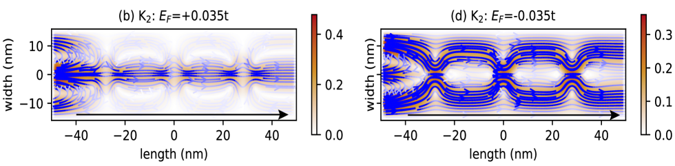
This image consists of two side-by-side scientific plots (labeled **b** and **d**) representing physical simulations of current flow in a nanostructure. The plots utilize heatmaps to show magnitude and blue streamlines with arrows to indicate the direction and density of flow.
---
## 1. Component Isolation: Plot (b)
### Header Information
* **Label:** (b)
* **Title:** $K_2: E_F = +0.035t$
* **Physical Context:** Represents a state with positive Fermi energy ($E_F$).
### Axis and Scale
* **Y-axis (Left):** labeled "width (nm)". Scale markers at -10, 0, 10.
* **X-axis (Bottom):** labeled "length (nm)". Scale markers at -40, -20, 0, 20, 40.
* **Color Bar (Right):** Vertical scale representing magnitude.
* **Range:** 0.0 to 0.4 (units unspecified, likely normalized current density).
* **Color Gradient:** White (0.0) $\rightarrow$ Light Orange $\rightarrow$ Dark Brown/Rust (0.4).
### Data Trends and Flow Analysis
* **Spatial Distribution:** The highest intensity (darkest orange) is concentrated along the central horizontal axis (width = 0) and at the far left entrance.
* **Flow Pattern:** Blue streamlines originate from the left ($x \approx -50$) and move toward the right.
* **Trend Verification:** The flow is highly collimated along the center. There are periodic "nodes" or narrowing points along the center line at approximately $x = -30, -5, 20,$ and $45$.
* **Peripheral Activity:** Outside the central channel, the streamlines form faint, recirculating vortices or "eddies" in the regions where the heatmap is white/light (low magnitude).
---
## 2. Component Isolation: Plot (d)
### Header Information
* **Label:** (d)
* **Title:** $K_2: E_F = -0.035t$
* **Physical Context:** Represents a state with negative Fermi energy ($E_F$).
### Axis and Scale
* **Y-axis (Left):** labeled "width (nm)". Scale markers at -10, 0, 10.
* **X-axis (Bottom):** labeled "length (nm)". Scale markers at -40, -20, 0, 20, 40.
* **Color Bar (Right):** Vertical scale representing magnitude.
* **Range:** 0.0 to 0.3 (Note: The peak scale is lower than plot b).
* **Color Gradient:** White (0.0) $\rightarrow$ Light Orange $\rightarrow$ Dark Brown/Rust (0.3).
### Data Trends and Flow Analysis
* **Spatial Distribution:** Unlike plot (b), the high-intensity regions (orange) are split into two parallel channels above and below the center line, roughly at width $\approx \pm 5$ nm. The center line (width = 0) shows low intensity (white).
* **Flow Pattern:** Blue streamlines are much denser and more widespread than in plot (b).
* **Trend Verification:** The streamlines exhibit a "braided" or "cellular" appearance. They diverge from the center at the entrance and follow the two outer paths, periodically pinching inward at $x \approx -25, 0, 25$.
* **Comparison:** This plot shows a clear "hollow" center in terms of current density magnitude compared to the "solid" center in plot (b).
---
## 3. Summary Table of Extracted Labels
| Feature | Plot (b) | Plot (d) |
| :--- | :--- | :--- |
| **Fermi Energy ($E_F$)** | $+0.035t$ | $-0.035t$ |
| **Max Scale Value** | 0.4 | 0.3 |
| **Primary Flow Path** | Central (width = 0) | Bifurcated (width $\approx \pm 5$) |
| **X-axis Range** | -50 to 50 nm | -50 to 50 nm |
| **Y-axis Range** | -15 to 15 nm | -15 to 15 nm |
## 4. Embedded Annotations
* **Directional Arrows:** Both plots contain a long black arrow at the bottom pointing from left to right, explicitly indicating the global direction of transport/length.
* **Streamline Arrows:** Small blue arrowheads are embedded within the blue lines to show local vector direction. In both plots, the net flow is from left to right, though local curvatures exist.